TauZero InterstellarPropulsion 2018

Breakthrough Propulsion Study Assessing Interstellar Flight Challenges and Prospects

Prepared by:

NASA Grant No. NNX17AE81G First Year Report

Marc G. Millis, Jeff Greason, Rhonda Stevenson Tau Zero Foundation Business Office: 1053 East Third Avenue Broomfield, CO 80020

NASA Headquarters, Space Technology Mission Directorate (STMD) and NASA Innovative Advanced Concepts (NIAC) Washington, DC 20546

Prepared for:

June 2018

pg 1 of 69

Millis 2018 Grant NNX17AE81G_for_CR.docx

This work was supported by NASA under grant No. NNX17AE81G, under the direction of Dr. Jay Falker, Jason Derleth, and Dr. Mike LaPointe of NASA Headquarters. The authors would like to acknowledge their encouragement and support for this effort.

Additional assistance came from Jim Gilland of the Ohio Aerospace Institute, Paul Gilster of the Tau Zero Foundation, Les Johnson of NASA, and the staff who helped run the 2017 Tennessee Valley Interstellar Workshop.

Any opinions, findings, and conclusions or recommendations expressed in this material are those of the authors and do not necessarily reflect the views of the National Aeronautics and Space Administration.

Progress toward developing an evaluation process for interstellar propulsion and power options is described. The goal is to contrast the challenges, mission choices, and emerging prospects for propulsion and power, to identify which prospects might be more advantageous and under what circumstances, and to identify which technology details might have greater impacts. Unlike prior studies, the infrastructure expenses and prospects for breakthrough advances are included. This first year’s focus is on determining the key questions to enable the analysis. Accordingly, a work breakdown structure to organize the information and associated list of variables is offered. A flow diagram of the basic analysis is presented, as well as more detailed methods to convert the performance measures of disparate propulsion methods into common measures of energy, mass, time, and power. Other methods for equitable comparisons include evaluating the prospects under the same assumptions of payload, mission trajectory, and available energy. Missions are divided into three eras of readiness (precursors, era of infrastructure, and era of breakthroughs) as a first step before proceeding to include comparisons of technology advancement rates. Final evaluation “figures of merit” are offered. Preliminary lists of mission architectures and propulsion prospects are provided.

pg 2 of 69

ABSTRACT

ACKNOWLEDGMENTS

Millis 2018 Grant NNX17AE81G_for_CR.docx

LIST OF TABLES …5

LIST OF FIGURES…5

ACRONYMS …5

EXECUTIVE SUMMARY…6 1.1. At-a-glance highlights in this report… 6 1.2. Content by Section … 6

INTRODUCTION …8 2.1. Provocations … 8 2.2. Objective and Approach… 9 2.2.1. Stage I - Defining the Problem as a Work Breakdown Structure (WBS) … 10 2.2.2. Stage II - Comprehensive Update to Interstellar Challenges & Prospects WBS … 11 2.2.3. Stage III - Remaining Analysis and Recommendations… 11 2.3. Outside Scope of Study … 11

PRIMER ON THE DISTINCTIONS OF INTERSTELLAR FLIGHT … 12 3.1. Distance… 12 3.2. Timescales… 15 3.3. Energy … 16 Infrastructure Dependence … 18 3.4.

INTERSTELLAR TECHNOLOGY CHALLENGES (Top-Down)… 19 4.1. Payload Challenges… 19 4.2. Propulsion & Power Challenges… 20 Incremental and Affordable Infrastructure Creation… 21 4.3.

PROPULSION & POWER PROSPECTS (Bottom-Up)… 22 5.1. Historical Spacecraft Baselines … 22 5.2. Proposed Interstellar Mission-Propulsion Architectures… 23 5.3. Propulsion & Power Concepts … 24 5.4. 2017 Workshop Review… 27

PROPOSED WORK BREAKDOWN STRUCTURE (WBS) … 28 6.1. WBS Hierarchical List … 28 6.2. Basic Analysis Flow Diagram … 29 6.3. List of Variables … 31

MEASURING MISSION CHOICES (Top-Down) … 33 7.1. Destination … 33 7.2. Mission Ambition … 33 7.2.1. Arrival Trajectory… 33 7.2.2. Science Sought … 34 7.3. Timing… 35 7.4. Motive … 37 7.5. Figures of Merit… 37

METHODS FOR EQUITABLE COMPARISONS … 39 8.1. Distinct Eras of Interstellar Flight … 39 8.1.1. Era of Precursors … 39

TABLE OF CONTENTS

pg 3 of 69

Millis 2018 Grant NNX17AE81G_for_CR.docx

8.1.2. Era of Infrastructure … 39 8.1.3. Era of Breakthroughs… 40 8.2. Baseline Mission & Payload Scenarios… 40 8.2.1. Solar Gravitational Lens … 41 8.2.2. Deep Interstellar Medium… 41 8.2.3. Centauri Flyby… 41 8.2.4. Centauri Slower Flyby … 41 8.2.5. Centauri Orbiter… 41 8.3. Measuring Infrastructure Dependence … 42 8.3.1. Earth-‐Based Beaming Infrastructure… 42 8.3.2. Estimating In-‐Space Infrastructure Availability and Growth… 43 8.3.3. Estimating In-‐Space Infrastructure Usage… 44 8.4. Measuring Disparate Propulsion & Power… 45 8.4.1. Type IP-‐OM: Internal Power & Onboard Reaction Mass … 45 8.4.2. Type RP-‐OM: Received Power & Onboard Reaction Mass… 48 8.4.3. Type RP-‐XM: Received Power & External Reaction Mass… 49 8.4.4. Type IP-‐XM: Internal Power & External Reaction Mass … 51 8.5. Estimating Comparative Rates of Advancement … 53 8.5.1. Baseline Performance Trends… 53 8.5.2. Technology Maturation Rates … 54 8.5.3. Modeling Technology Advancement Rates in General… 56 8.5.4. Other Methods Under Consideration… 57

SAMPLE DATA PLOTS … 59 9.1. Technology Comparisons … 59 9.2. Mission Comparisons… 60

STAGE II PLANS … 62 10.1. Collection and Display of Information from Subject Matter Experts … 62 10.2. Analysis Portal… 63 10.3. General Audience Website … 63 10.4. Concluding Remarks … 63

REFERENCES… 64 11.1. Sequentially Cited… 64 11.2. Bibliography… 65

pg 4 of 69

Millis 2018 Grant NNX17AE81G_for_CR.docx

Table 14. Alternative Progress Measures, Linking Performance, Schedule, and Cost … 58

Destinations of Interest, Including Potentially Habitable Exoplanets … 14

Historic Exploration Mission Baselines… 22

Interstellar Mission-Propulsion Architecture Concepts … 23

Power and Propulsion Prospects … 26

2017 Workshop Lectures & Authors … 27

List of Variables … 31

Arrival Trajectory Options … 33

Time on Target Verses Flyby Speed… 34

Span of Motivations, Consequences, and Provisional Rankings … 37

In-Space Infrastructure Availability and Growth Estimating … 43

Power & Propulsion Analysis Types … 45

Tracking the Advancement Trends of Common Technologies … 54

Technology Maturation Levels and Relative Durations Between Them … 55

Table 9.

Table 8.

Table 7.

Table 6.

Table 5.

Table 4.

Table 3.

Table 2.

Table 1.

Table 13.

Table 12.

Table 11.

Table 10.

Figure 1.

Figure 2.

Figure 3.

Figure 4.

Figure 5.

Figure 6.

Figure 7.

Figure 8.

LIST OF TABLES

LIST OF FIGURES

ACRONYMS

Millis 2018 Grant NNX17AE81G_for_CR.docx

pg 5 of 69

Attitude Control System Artificial Intelligence Breakthrough Propulsion Physics

ACS NASA Innovative Advanced Concepts NIAC AI Power Management and Distribution PMAD BPP RF Radio Frequency (Electromagnetic Waves) C&DH Control and Data Handling RP-OM Received Power - Onboard Reaction Mass Calendar Year CY RP-XM Received Power - External Reaction Mass European Southern Observatory ESO Radioisotope Thermal Generator RTG Faster Than Light FTL Space Mission Technology Directorate SMTD Guidance Navigation and Control GNC Scientific Readiness Levels SRL Technology Readiness Levels Internal Power - Onboard Reaction Mass IP-OM TRL Tennessee Valley Interstellar Workshop TVIW Internal Power - External Reaction Mass IP-XM Work Breakdown Structure Journal of the British Interplanetary Society WBS JBIS

Topological Assessment Process in Principle… 9

Correlating Interstellar Distances with Human Timescales and Flight Speeds … 13

Timescale of Interstellar Missions and Historic Technology Advances … 15

Interstellar Mission Energy Versus Available Energy… 17

Basic Analysis Flow Diagram … 30

“First Image” Examples from History (Luna 3 and Mariner 4) … 35

“S-Curve” Pattern of Technology Advancement … 56

Technology Comparison Plots (a, b, c)… 60

Figure 9. Mission Comparison Plots (a, b, c) … 61

1. EXECUTIVE SUMMARY

Dozens of interstellar mission concepts have been published that are based on known physics—and dozens more will be published in the future. All of the concepts require the maturation of one or more technologies or the building of infrastructure—or both. The US is not ready to launch a genuine interstellar mission, but is ready to start making investments to get ready to launch a mission within a few decades. The investment of limited resources will be required to get from where we are today to a future of interstellar travel. Careful selection of where to invest the resources is essential.

Choosing which concepts to fund requires the comparison of very different approaches. A challenge is to compare technologies as disparate as a fusion rocket and a ground-based laser pushing on a sail. In addition, not all of the proposed approaches to interstellar travel rely entirely on known physics. Champions of various technologies have a tendency to focus only on what is good about a given concept, sans implications for a complete system design. Therefore, an additional motivation for our metrics is to help identify “if it is real, would it also be useful?”

Many of the concepts of interest could revolutionize travel within the solar system, in addition to getting us closer to interstellar travel. Thus, investing in mission concepts that can both be employed usefully in near-term missions and be on the roadmap to future interstellar missions is of high interest.

This report derives figures of merit based on the physics of propulsion technologies and other mission factors. The metrics will allow policymakers to make decisions about which technologies would be more valuable, and to identify the subset of technologies that would do double-duty by enabling both longer-term interstellar missions and ambitious nearer-term missions.

At its foundation, these metrics rely on three core parameters: 1) how much energy will be expended, 2) how long does it take to perform a mission, and 3) distance traveled. It’s like comparing modes of transportation: an airplane is faster than a car, but travel by car uses less energy and is therefore cheaper. Mission funding can compare the energy it will take versus a scientific objective (such as destination of interest) versus how long it will take to get the data.

1.1. At-a-glance highlights in this report

Flowchart to guide a user in applying the assessment of a technology: Section 6.2, page 30.
Sample data plots using the methodology with hypothetical technologies: Section 9, pages 60-61.

pg 6 of 69

Section 4 identifies problems of interest that will be needed to make interstellar travel attainable, such as

Section 5 is a wide-ranging list of technological approaches identified from the literature for how to solve

propulsion, power, and data transmission.

the problems—to be evaluated in Stage II.

Section 6 organizes the metrics into a work breakdown structure, and provides a flowchart to guide a user

in applying the assessment of a technology.

Section 7 summarizes key mission choices and variables that must be defined in order to assess a mission approach—such as where is the mission going, how long will it take to get there, how much data will be returned, and type of mission: fly-by or orbiting.

Section 8 lays out the comparison metrics for how dissimilar mission concepts can be quantitatively compared in an equitable manner. The process defines four different propulsion types according to their source of power and reaction mass (internal or external). Each type requires different analyses, where their unique performance measures are converted into the more general measure of energy.

1.2. Content by Section

Section 2 reviews the background and objectives of this study.

Section 3 provides a technical background about interstellar travel.

Millis 2018 Grant NNX17AE81G_for_CR.docx

Section 9 shows examples of data charts based on the methods of Section 8. At this stage the comparisons are only with hypothetical propulsion technologies to test the methods and plotting options. These will be further refined in Stage II.

Section 10 discusses Stage II of this project.

Section 11 provides a list of references.

Millis 2018 Grant NNX17AE81G_for_CR.docx

pg 7 of 69

2. INTRODUCTION

Interstellar destinations are about three orders of magnitude farther away than can be reached using current technology. Many advanced propulsion concepts have been conceived, but their performance predictions are not yet certain enough to be ranked reliably using traditional trade studies. Further, the mission architectures in which these concepts were proposed used different assumptions that make equitable comparisons impossible.

There have been several overviews of the challenges and prospects of interstellar flight, most notably starting with the 1976 interstellar exploration program proposed to congress [1], the 1989 Starflight Handbook [2], the 1992 Prospects for Interstellar Travel [3], 2001 “Interstellar Flight Primer” [4], and the 2004 Centauri Dreams [5]. Among the large number of technical papers, several volumes of the Journal of the British Interplanetary Society were devoted to interstellar flight [6-8]. There has not, however, been an impartial, overall evaluation of the prospects and related next research steps.

There is a need for a new assessment method that can compare the uncertain, long-term prospects of emerging technology for interstellar flight. The assessment method must be able to equitably compare concepts that use entirely different propulsion methods (sails, rockets, and others). The comparisons should show which concepts might be the most advantageous and under what conditions, plus identify the most impactive supporting technologies. Further, given the long timescales of interstellar flight, the assessments should have provisions for considering advances that might reach fruition over decades of further advancement. And finally the assessments should suggest a prudent portfolio of next-step research.

2.1. Provocations

pg 8 of 69

The impetus for this study dates back to a 2006 workshop held at Princeton University. As with prior interstellar sessions, various propulsion and mission concepts were presented as if to advocate their selection [9]. In the subsequent discussions, it was agreed that it was not possible to pick a winner. Each concept used different assumptions, plus the performance predictions are unproven. Rather than attempt far-future decisions, the discussion turned to identifying the most critical make-break questions for each approach, and of those, which can be affordably researched next. Pursuit of these questions shaped the goals and strategies of the nonprofit Tau Zero Foundation that was incorporated that same year [10].

Interest in interstellar flight is increasing. The continuing discovery of exoplanets, the announcements of privately funded mission plans, and the inkling that faster-than-light flight is now at least theoretically possible, provokes more interest. The following paragraphs describe some of the more significant provocations, in chronological order.

Theories for faster-than-light (FTL) flight are now part of the scientific literature. The first traversable wormhole article was published in 1988 [11], the first warp drive paper in 1994 [12], and the first scholarly book compiling these challenges along with other breakthrough propulsion pursuits was published in 2009 [13]. Even the hint that FTL might someday be possible, makes interstellar flight more attractive.

In 2014, the first potentially habitable Earth-size exoplanet (Kepler-186f, ≈ 500 ly) was confirmed by the Keck and Gemini Observatories. Now it is certain that potentially habitable planets exist, perhaps even Earth-like planets [14].

In April 2016, an ambitious plan for an interstellar mission was announced, with an offering of $100 Million for its initial research from Russian billionaire, Yuri Milner. The project, called “Breakthrough StarShot,” is based on using a powerful laser array to push a small light-sail up to 20% lightspeed to reach Alpha Centauri within a 22 year flight time [15]. This project continues to receive significant media attention, further amplifying public interest in interstellar flight.

And in August of 2016, a potentially habitable exoplanet, Proxima b, was discovered orbiting our nearest neighboring star, Proxima Centauri, at only 4.2 ly distant [16]. Though subsequent analysis casts doubt that the planet could support human life, due to the intense radiation from its sun, the fact that our nearest neighboring star hosts an exoplanet that is roughly similar to Earth’s size and temperature spurs further interest in the search for habitable worlds.

Congressional interest followed. An 18 May 2017 report for the fiscal 2017 Appropriations Committee included the following instructions: “The Committee encourages NASA to study and develop propulsion concepts that could enable an interstellar scientific probe with the capability of achieving a cruise velocity of 0.1c. These efforts shall be

Millis 2018 Grant NNX17AE81G_for_CR.docx

centered on enabling such a mission to Alpha Centauri, which can be launched by the one-hundredth anniversary, 2069, of the Apollo 11 moon landing.” [17].

2.2. Objective and Approach

The objective of this study is to create a process for equitably comparing different mission architectures and possible propulsion and power technologies, in order to determine which research paths have the greatest leverage for improving NASA’s ability to explore farther, faster, and with more flexibility. The specific goal of achieving 10% lightspeed was included by Congress, and it is likely that this goal will require the combination of a number of different technologies to succeed. The more exact questions that arise from further analysis are: which elements of that goal have more leverage toward success, and what knowledge gaps remain to solve each of those problems?

Toward that end, the process shall establish common performance measures for the disparate propulsion and power approaches, and accommodate the uncertainty in the performance predictions. The comparisons will include the scale of infrastructure needed to build and launch interstellar missions, include consideration of potentially disruptive advancements for spaceflight, and suggest how to plan a research program that systematically seeks the most desirable of such advancements.

In contrast to mission trade studies that seek the best technology to meet a set of well-defined requirements, this study will use topological analyses. Topological methods have been devised recently to compare general goals to broad technology areas to produce “topological maps” that identify research areas of potentially greater impact (instead of creating “road maps” to develop a specific technology) [18, 19]. These tools can determine the sensitivity of mission choices to performance requirements, as well as determining which technologies have greater impact on meeting those requirements (e.g. common elements of more than one subsystems). Figure 1 shows this analysis process in principle, and where the example maps are from Gilland [19].

In support of the general topological comparisons, more deterministic analyses are also developed. This

includes the equations to convert the varied propulsion performance measures into common figures of merit.

Since the timescales for interstellar flight are comparable to historic examples of the emergence of breakthrough technologies, it is desired to include promising long-range research whose prospects are still speculative and whose mission impacts cannot yet be quantified. Presently, the practice is to wait until new prospects emerge on their own in a form ready to be evaluated per the familiar mission trade studies. However, this “wait and see” posture lets potentially revolutionary advances languish with little progress.

Process in Principle Topological Analysis

pg 9 of 69

Vary inputs to explore consequences

Choice-Driven Inputs *  Launch year (baselines) *  Destination *  Mission duration or speed *  Data return duration *  Mission ambition *  Motive weighting factors *  Readiness thresholds *  Performance thresholds *  Scale of research support *  Scale of mission effort

Relative Influence

Prospects Now & Future *  Mission Architecture Options Specs *  Power & Propulsion Options Specs

Nature-Driven Challenges *  Distance, Energy = f (m, ∆v), etc. *  Physics Performance Limits

Fig. 1a. Inputs to Determining Topological Maps Gilland (2013) Aspects of Technology Program Planning: Top-Down to Bottom-Up

Millis 2018 Grant NNX17AE81G_for_CR.docx

Fig. 1b. Example Map, Missions & Requirements

Fig. 1c. Example Map, Technologies & Research

pg 10 of 69

Fig. 1. Topological Assessment Process in Principle

To search for such latent prospects, this study will include the topic of breakthrough propulsion physics. The term “breakthrough propulsion physics (BPP)” comes from the NASA project by that name which examined non- rocket spacedrives, gravity control, and faster-than-light travel [20]. In contrast to technological advancements rooted in known physics, BPP pursues entirely new technologies from further advances in physics. The grounding reference for this portion of the study is the book, Frontiers of Propulsion Science [13].

The first step of the scientific method is to define the problem. Similarly, this study will begin with an assessment of the challenges and prospects in a manner suitable to the unique situation of interstellar flight. Sponsored by a multiyear NASA grant NXX17AE81G, this “Breakthrough Propulsion Study” is divided into three stages, 1) defining the problem, 2) collecting information, and then 3) analytical testing.

The scope of this report covers the first stage of this study: defining the problem of tracking, assessing, and

planning the most effective research paths to reach the stars.

2.2.1. Stage I - Defining the Problem as a Work Breakdown Structure (WBS)

The challenges of interstellar flight and the technological prospects for answering those challenges are examined to determine how to proceed later with a fully-rigorous and impartial assessment. Or, in other words, this stage aims to ask the right questions.

2.2.1.1. Challenges - Top Down Mission Awareness The prior goals from interstellar studies will be refined to encompass a more complete set of factors - in short to understand the whole problem before suggesting solutions. Recent investigations of interstellar prospects found: 1) mission motivations are often implicit and limited in scope, 2) vehicle concepts often neglect the interplay with the infrastructure needed to build, power, and launch the vehicle, and 3) the major impediments to interstellar flight are less about technological prowess than about limitations of energy, where it appears that roughly two centuries remain before sufficient energy is likely to be available to launch an interstellar mission, regardless of the choice of flight method [21]. Note, however, that the uncertainty bands of those estimates are substantial.

2.2.1.2. Prospects—Bottom Up Technological and Scientific Principles A wide span of interstellar flight prospects, from the basic solar sail all the way to the speculative FTL flight will be included to 1) provide a cursory understanding of their projected performance, and 2) devise methods to convert their disparate performance measures into common terms. Though the options use a widely varying range of parameters to describe their performance, energy is chosen as the central measure for this commonality. In essence, energy is the fundamental currency of all motion.

Millis 2018 Grant NNX17AE81G_for_CR.docx

With the participation of Tau Zero Personnel, the “Tennessee Valley Interstellar Workshop (TVIW)” was convened in October of 2017 to gain an up-to-date summary of the projections and status of interstellar flight options and issues, discussed in Section 5.4.

In this report, the combination of challenges and prospects are used to create a new WBS to collect the complex information in an organized manner. A set of variables corresponding to that WBS are defined to guide the information collection process of Stage II. This will be expanded to identify which operating parameters of the different propulsion and power methods will need to be collected to continue the analysis.

While the focus of this first stage is the development of the overall structure for the data to be subsequently collected in later phases, some values have been specified as starting estimates, for which more accurate and defensible numbers are sought. If readers have more accurate numbers for any of these values, please contact the authors with that information along with a reference citation for those more accurate values. Further, note that most values herein are specified to only about two significant digits—consistent with the current fidelity of interstellar flight estimates.

2.2.2. Stage II - Comprehensive Update to Interstellar Challenges & Prospects WBS

In Stage II, a web-based system will be created to allow subject matter experts from around the globe and from the span of relevant disciplines, to populate the WBS with their most recent data. Early drafts of technology development roadmaps will begin, with the intent to impose consistent methods of estimating the development durations.

The initial equations and analysis process will be refined, including running test cases with illustrative missions,

payloads, and propulsion types. From there, the topological analysis methods will be adapted to this problem.

2.2.3. Stage III - Remaining Analysis and Recommendations

Stage III is where the analyses will be iteratively run and refined to ensure that it is meeting the needs of NASA and the interstellar flight community. The analyses should show which concepts might be the most advantageous, plus identify the most impactive supporting technologies. This includes identifying which knowledge gaps have the highest potential for improving the technology, and then how to solicit research to fill those gaps. This includes prospects for disruptive advancements and ancillary influences. And finally, the assessments will suggest a prudent portfolio of next-step research.

Once completed, technology roadmaps can be devised that are rooted in common standards to allow fair

pg 11 of 69

There are two activities related to interstellar flight whose assessments and recommendations are beyond the

scope of study, “interstellar precursor missions,” and “world ships.”

Interstellar precursor missions are those that can be launched from Earth using foreseeable spacecraft technology and without needing substantial new infrastructure [22-33]. By “foreseeable technology” it is meant those technologies that are mature enough for mission trade studies. This study instead focuses on longer-term and farther-reach technologies whose performance measures are less certain. These precursor missions will, however, be used in this study as performance baselines and scaling examples. Further progress on precursor trade studies are a valuable aid to these longer-range interstellar flight assessments. An example of a precursor mission that would help resolve questions for future interstellar mission planning is the concept of a “Look-Back Mission.” A look- back mission would test a suite of exoplanet instruments by looking back toward Earth at various distances to determine the effect of viewing distance and time on target for collecting meaningful information.

Another group of mission and technology concepts which are beyond the scope of this study are “world ships” - concepts for multi-generation, self-sustaining colonies of humans living aboard spacecraft headed toward potentially habitable exoplanets [34]. Even though such goals address the important motive of the sustained survival of humanity, they are out of scope since their major research goals involve sustainable habitats and cultures instead of propulsion.

comparison of one roadmap to the other.

2.3. Outside Scope of Study

Millis 2018 Grant NNX17AE81G_for_CR.docx

3. PRIMER ON THE DISTINCTIONS OF INTERSTELLAR FLIGHT

Interstellar flight is far more challenging than any prior space mission. The distances, timescales, and energy levels of interstellar flight are beyond precedent. In colloquial terms, interstellar distances are so vast that they make lightspeed seem slow. This section offers a preview of these differences to set the context for the assessments that follow.

3.1. Distance

pg 12 of 69

Voyager has traveled farther than any other spacecraft to date, yet it has traveled less than one-thenth of one percent of the distance to Proxima Centauri (142 AU by 2018, 0.053% of 270,000 AU). It took Voyager over four decades to reach that distance and would take another 80-thousand years to span the distance equal to reaching the Centauri stars (velocity ~ 0.00006 c). The farthest conceivable missions based on contemporary technology could only reach less than a half-percent of the way to Proxima Centauri in 50 years (1000 AU, 0.37% of 270,000 AU) [32].

In addition to the challenge of raw distance, there is the challenge of how much distance there is between interesting destinations. The logarithmic scales used in figure 2, and similar charts from other studies, can be misleading when trying to grasp the true scale of interstellar destinations. When plotted on logarithmic scales, it appears that destinations of interest are spread evenly. When listed linearly however, the vast gaps between points of interest become more apparent. If a chart encompassing the distance to our nearest star spanned the full height of this report’s margins (270,000 AU ≈ 23 cm, 9”), then the maximum distance achievable within a 50 year flight time using existing technology would only barely distinguishable from the chart’s origin (1000 AU ≈ 1 mm ≈ 1/32”).

Table 1 lists interstellar destinations by distance along with other factors that come into play in later parts of this report. Note in particular the column “ESI,” which stands for “Earth Similarity Index,” from the “Planetary Habitability Laboratory” at the University of Puerto Rico at Arecibo. An ESI of 1.00 would be fully Earth-like. The other key destinations are as follows. The edge of our solar system can be defined as beyond around 200 AU. The next destination of interest past that point is 550 AU, where the gravitational lensing effect of our sun can be used to magnify images of whatever is on the opposite side of the sun [36]. It has been proposed that this solar gravitational lens has the magnification to be able to image an exoplanet with enough resolution to distinguish land features [37].

Beyond that point, the next targetable object is almost 500 times farther away, specifically the Centauri star systems (270,000 AU, 4.2 ly). In the vast void between those points of interest there exist only sparse densities of comets and asteroids; the Hills cloud (2,000 AU), Oort cloud (10,000 AU), and the G-cloud (41,000 AU) [38]. These features are difficult to discern using Earth-based astronomy, but probes passing through them could make direct in-situ measurements of the fields and particles.

Once past the Centauri systems, there are already eight potentially habitable planets detected within 41 ly, half of which are within 22 ly. Based on the astronomical data available before 2010, Claudio Maccone created statistical estimates for how far away the nearest Earth-like planet might be, and how far away the closest extraterrestrial civilizations might be. The distance estimates to the closest Earth-like planet span roughly 50 ly to 100 ly. The distance estimates to the nearest possible civilization are beyond 2000 ly [39]. Though these are rough statistical estimates, they at least help convey the scale of the challenge.

Another aspect of distance is time—how far can be reached within human timescales and the ultimate longevity of spacecraft. A common mission duration cited for interstellar concepts is 50 years, perhaps based on a long career span where the people who launched the mission will still be able to witness its findings. There has not been a study to assess the limits of human patience for interstellar missions.

There has also not been a study to estimate the longest possible operating duration for a space probe, yet 200

years is a fair starting estimate. Thus, even at lightspeed, the farthest a probe could reach into our galaxy is 200 ly.

Millis 2018 Grant NNX17AE81G_for_CR.docx

l l i

e g d e

s n e L

s i h t

r e l p e K

t u o h t i

e s e i l

n i a m e r

w e n o z

t s i p p a r T

b a m i x o r P

l a n o i t a t i v a r G n u S

. e l b i s s e c c a n i

, t h g i ﬂ t h g i l

n a h t

r e t s a f

l a n o i t a r e p o t f a r c e c a p s

h t r a E

s l i o B h t r a E

y r u t n e C

r y n o i l l i

a i n n e l l i

e d a c e D

h t n o M

e l b a b o r P

r a e Y

k e e

r y

i l

t i

Millis 2018 Grant NNX17AE81G_for_CR.docx

pg 13 of 69

U A

Fig. 2. Correlating Interstellar Distances with Human Timescales and Flight Speeds

Figure Caption: This figure shows the correlation between long timescales, interstellar distances, and average flight speed. Both the distance and timescales are logarithmic. The horizontal scale spans the radius of the Milky Way galaxy (50,000 ly), while the time scale extends all the way to the certain end of Earth’s habitability (~1 billion years [35]). The assumed upper limit for the operational duration of a space probe (200 years) is shown. The diagonal lines represent different speeds, starting on the left with Voyager’s 0.00006 c. The faster Juno spacecraft (0.00025 c) is also shown. The other diagonal lines are in terms of fractional lightspeed, shown in increasing factors of 10 all the way up to lightspeed. For each factor of 10 increase in speed, the required energy goes up by at least a factor of 100.

Table-1 Destinations of Interest, Including Potentially Habitable Exoplanets.

Level of Interest Score (Subjective). Values shown are starting points for discussion and resolution. (Di) Type 100% 80% 5% 10% 10% 5% 50% 5% 10% 80% 80%

Destination irrelevant “µEarth ship,” “Colony Ship,” “World Ship” Interstellar Asteroid: long aspect ratio object through solar system ≈5 AU/yr Origin of most short period comets. 100,000 icy objects > 100 km diam. Dwarf planet Dwarf planet Transition from our solar system toward the galactic background Historical artifact, long duration exposure evidence Fully outside our solar system Hypothesized, farthest planet of our solar system Maccone 1998 Turyshev 2017, TVIW Milestone, 1000 AU (TAU)

ESI*

20,000

m e t s y S

r a l o S n I

m u i d e M

AU start

ly start

r a l l e t s r e t n I

Distance (Dd)

? Exo Image

Interest Factors

90% 85% 70%

Destinations (Dn)

Extends to

98 1,000

0.001 0.002 0.016

Description, Relevance

0.316 0.000 0.316 3.163

5% 5% 5% 15% 5%

20,000 200,000 0.7 ly

Proxima Centauri Alpha Centauri A & B Barnard’s Star

Hills Cloud (Torus) (?) VLIM LISM Oort Cloud sphere (?) G-Cloud ??

µEarth Ships Placeholder “Oumuamua” object Kuiper Belt Eris Sedna Heliopause Voyager Spacecraft Interstellar “wind” Planet Nine (?) Solar grav’ lens start Solar grav’ lens nominal

Observable Biomarker? GJ 682 HD 20794, 82 G Eridani Gliese 581 Gliese 832 Gliese 667 GJ 1132 Trappist-I LHS 1140 Nearest hab exoplanet?

Epsilon Eridani Procyon Tau Ceti GJ 273 Gliese 191 (Kapteyn b) Wolf 1061 Gliese 687 Gliese 876

≈ 3 AU in 2017 +5AU/yr**

0.0005

0.001

0.002

0.003

0.004

0.009

0.010 1,000 0.016 2,000 0.032 2,063 0.033 3,000 0.047 10,000 0.16 3.8E+04 0.60 6.3E+04 1.0 1.0E+05 1.6 2.7E+05 4.2 2.7E+05 4.3 3.8E+05 6.0 5.0E+05 7.9 6.3E+05 10.0 6.6E+05 10.5 7.2E+05 11.5 7.6E+05 12.0 7.8E+05 12.4 8.2E+05 13.0 8.7E+05 13.8 9.3E+05 14.7 9.7E+05 15.3 1.0E+06 15.8 1.0E+06 16.0 1.0E+06 16.6 1.3E+06 19.8 1.3E+06 20.3 1.3E+06 21.0 1.4E+06 22.0 2.5E+06 39.3 2.5E+06 39.5 2.6E+06 40.7 4.4E+06 70.0 6.3E+06

1.4E+07

3.5E+07

4.9E+07

6.3E+07

7.1E+07

7.6E+07

1.3E+08

2E+09

Kepler 442 Kepler 62 ET Civilization? To Center of Galaxy

ESI = Earth Similarity Index: http://phl.upr.edu/projects/habitable-exoplanets-catalog/results ** In comparison, Voyager is ≈ 3.5 AU/yr, and Juno ≈ 15.5 AU/yr

N/A 80% 80% 80% 80% 95% 90% 95% 95%

80% 10% 80% 80% 85% 80% 80% 80%

K2-72 Kepler 186 Kepler 1229

Yellow refers to distance numeric milestones

Milestone, 1000 light-years

100% 100% 100%

pg 14 of 69

95% 100%

.61 f .73 b

.84 b .67 f

s t e n a l p o x E

? e l b a t i b a H

? d e t i b a h n I

t s e r a e N

Very Local Interstellar Medium [McNutt 2016] Local Interstellar Medium [McNutt 2016] Far enough to compare parallax to Hubble red-shift distance (basic physics) Next transition into local interstellar medium ? Milestone, 1 light-year Milestone, 100,000 AU

.85 b Closest hab-cat exoplanet. Red-Dwarf (M5.5V), 1 planet in HabZone (b) A is like our Sun; B is spectral type K2, Maybe 2 planets around B Project Daedalus target. Low-mass red dwarf No exoplanets confirmed. Milestone, 500,000 AU Milestone, 10 light-years K2 star, similar planetary system to a young Sun. Unconfirmed exoplanet (b) Binary system with white dwarf star Closest lone star similar to sun Unconfirmed 2 of 5 planets in HabZone (e, f) M3.5 star. 1 of 2 planets in HabZone (b) .67 b M1.0 star. 1 of 2 planets in HabZone (b) M3.5 star. 1 of 3 planets in HabZone (c) M3V star. 1 of 1 planets in HabZone M4V star. 2 of 4 planets in HabZone (b,c) Milestone, 1-Million AU Predicted 2030 astronomy biomarker detection range [51] M3.5V star. 1 of 2 planets in HabZone (b) G8V star. 1 of 3 planets in HabZone (d) M2.5V star. 1 of 5 planets in HabZone (g) M1.5 star. 1 of 2 planets in HabZone (c)

.84 Cc M1.5 V (3-star system). 4 of 7 in HabZone (.84 Cc, .77Cf, .60 Ce) 3-ESI’s

M3.5 star. 1 of 1 planets in HabZone (b)

.85 e M8V star. 3 of 7 planets in HabZone ? (.85 e, .68 f, .58 g) MULTIPLE .68 b M4.5 star. 1 of 1 planets in HabZone (b)

Highest probable distance of nearest habitable planet [Maccone 2010] Milestone, 100 light-years

First discovered potentially “Earth-like” exoplanet

Probable distance of nearest extraterrestrial civilization [Maccone 2010]

Millis 2018 Grant NNX17AE81G_for_CR.docx

A mission takes longer than just the time to reach its destination. There is also the time-of-flight for the return signals to reach Earth, and the time it takes to finish transmitting the data. This last duration, transmit time, is not trivial. For example, at the extremely low power levels envisioned for the Breakthrough StarShot mission, it has been estimated that it will take 20 years to transmit the data [40]. Hence, the total mission duration for Breakthrough StarShot is roughly 46 years (22 yr trip, 4 yr signal delay, 20 yr transmit time).

For this study, “Total Mission Duration,” Tm, is defined as the sum of the “trip time,” Tt, to reach the destination, the “signal time,” Ts, for the data to begin to reach Earth, and the “transmit time,” Tx, to send the acquired data. Figure 3 shows a comparison between the projected timescales for precursor missions, the StarShot mission, and the mission suggested in the 2016 congressional language [17].

The timescales of some historic technological breakthroughs are shown for comparison on figure 3. For example it took only six decades from the discovery of natural radioactivity to having a nuclear power plant on the electrical grid (1890-1950). It took a little over two decades from the creation of the rocket equation to the first liquid rocket, and another four decades before humans walked on the moon (1903-1926-1969). Another fitting example is the 1-century between the steam power era, when Jules Verne wrote his fictional depiction of a Moon mission (1865) and the first actual lunar landing (1969). If scientists and engineers of the steam era were contemplating Moon missions, would they have debated which steam cycle to use, or perhaps even considered Verne’s cannons? What was missing at that time was the undiscovered future of electrical power, liquid rockets, and nuclear power. What is next in our undiscovered future?

Since the timescale for revolutionary technological developments are comparable to interstellar mission durations, the potential impact of future advancements are considered as part of this study. While it is not possible to predict the future with certainty, the historic patterns of technological revolutions can be used as guides for this study [41].

Timescale is Not Business as Usual

3.2. Timescales

History Lessons

Interstellar Medium

StarShot Centauri

Predictions

Congress?

100, Steam-era & Verne’s moon fiction (cid:1)︎ Apollo

60, Nuclear science (cid:1)︎ Grid power

Rocket equation (cid:1)︎ Liquid rocket

70, Light bulb (cid:1)︎ ENIAC

Transmit Data

Transit Centauri

? AI Ascension

Tech & Build

Technology

50 yr to 1000 AU

30 yr to 200 AU

2060

2080

2030

Build

D e a y

Predictability ?

B u

i l

pg 15 of 69

D a t a

Fig. 3. Timescale of Interstellar Missions and Historic Technology Advances

Side note: TVIW 2016 estimated it would take 4-centuries to build a world ship

There will also be unpredicted impacts from ancillary advances, such as from Artificial Intelligence (AI). Predictions of when AI will eclipse the capacity of the human mind (measured in “operations per second”) span from 2030 to 2050 [42]. Speculating, will the AI advancements solve the challenge of fully-autonomous probe operation? Will AI processors become able to more quickly (and impartially) devise and test “grand unification” theories—perhaps resolving the unknowns of new propulsion physics? Either of these would be a significant, positive impact. If such desired functionality is pursued, it will at least offer a more optimistic path for when AI eclipses human abilities.

⬅︎ Business as usual

⬅︎ Challenge

Transit Centauri 10%c

Extinction ?

Millis 2018 Grant NNX17AE81G_for_CR.docx

Another ancillary advancement that might impact the priorities behind interstellar flight is transhumanism, which means the continued merging of technology into the human body to enhance performance. Transhumanism has fewer scholarly articles from which to extract predictions and implications, yet it is already happening. Examples include dental fillings, eye glasses, hearing aids, pacemakers, replaced joints, cochlear implants, etc. Will this expand to making humans able to tolerate indefinite periods at low gravity, or able to enter synthetic hibernation to endure long space voyages? While only crude speculations at this time, the potential impact to watch for is a shift in priorities from probes to human journeys.

As much as continuing advances in science and technology will make it easier to launch an interstellar mission, these advances also create a quandary, the “Incessant Obsolescence Postulate”—no matter when an interstellar probe is launched, a subsequent probe will reach the destination sooner and with more modern equipment. This is only a postulate, not a theorem nor even a principle. It is presented here not as an immutable constraint, but as one of the assumed impediments for pursuing interstellar missions.

As an aside, the term, Incessant Obsolescence Postulate, was first coined by the author around 1999 [5 p.157]. This same notion has been called “catch me if you can” [43], the “incentive trap,” by Andrew Kennedy [44] and “Zeno’s paradox in reverse,” by David Brin (a term possibly originating during the 1994 workshop; “Interstellar Robotic Probes-Are we ready?” [43])

Although this Incessant Obsolescence Postulate might appear valid, it will eventually expire. Due to the combination of the nonlinear nature of both advancement trends and relativistic spaceflight, there will be a point where an optimum launch opportunity occurs [44,45]. Waiting longer does not get you to the destination sooner. Kennedy dubbed his optimization calculation the “wait equation” [44]. Approximately when missions begin to take less than a generation (20-30 years), there is no need to wait longer [45]. Conversely, when mission times are much longer, then investing in technology to improve mission time is a credible strategy.

In addition to the eventual expiration of incessant obsolescence, the most significant factor that renders it

irrelevant is if the motive is something other than being first, such as technology development.

3.3. Energy

pg 16 of 69

Trip time is a function of propulsion energy and payload mass. Higher speeds or greater spacecraft mass demand more energy. Following the kinetic energy equation (KE = ½m v2) as the lowest bound on required energy (where propellant mass and inefficiencies are ignored), doubling the spacecraft mass at least doubles the required propulsive energy. Doubling the velocity at least quadruples the required propulsive energy, since energy goes as the square of the velocity. Note, relativistic effects do not become significant (> 1.0%) until past 14% lightspeed.

One of the largest impediments to starflight is the gap between the energy required for propulsion and the energy available, regardless of the choice of propulsion. Calculations that compared the rate of humanity’s growing energy prowess to the energy required for propulsion suggest that perhaps two centuries remain before sufficient energy is likely to be available [21]. This estimate took into consideration that only a portion of total world energy would be allocated for space missions. By comparing the Space Shuttle launch history to the US energy capacity over the same years, an estimate for that allocation is found to be one-millionth. Granted, such a rough estimate could be off by an order of magnitude or two, which should be taken in consideration. Figure 4 shows that comparison from the 2010 paper (with revisions & corrections).

For an example of the magnitude of propulsion energy, consider the 1-gram StarShot spacecraft traveling at 20% lightspeed. Just its kinetic energy is approximately 2 TJ. When calculating the propulsive energy in terms of the laser power and beam duration, (100 GW for minutes) the required energy spans 18 to 66 TJ, for just one probe. The full suite of 1,000 probes would be 1,000 times that span. For comparison, the energy for that suite of 1,000 probes is roughly the same as 1-4 years of the energy consumption of New York City (NYC @ 500 MW).

If instead of a 1 g spacecraft, the kinetic energy is calculated using the mass of a Voyager type spacecraft (≈ 1,000 kg) traveling at 10% lightspeed, then the kinetic energy becomes 4.5 x 105 TJ. For comparison, this is about one-thousandth of the total world energy consumption in 2016 (5.5 x 108 TJ [46, 47]).

Millis 2018 Grant NNX17AE81G_for_CR.docx

) J (

1.E+15

1.E+19

1.E+18

1.E+17

1.E+16

d n a

e n O

l a b o l G

y g r e n E

l a u n n A

f o h t n o i l l i

r a l l e t s r e t n I

y g r e n E n o i s s i

1.E+13

1.E+14

Higher Growth 3.6%

Average Growth 1.9%

Lower Growth 0.2%

Calendar Year

2200

2400

(2) Ten Starshot Beam

(6) Rocket Rendezvous

(5) Rocket Flyby

(4) Probe Rendezvous

(3) Probe Flyby

pg 17 of 69

(1) Ten StarShot Kinetic

Fig. 4. Interstellar Mission Energy Versus Available Energy

Figure Caption: This chart compares the amount of energy likely to be made available for interstellar missions (one-millionth of total world energy) to the energy required for interstellar missions. The central diagonal line is the nominal energy growth from extrapolating data spanning 1980-2007. The upper and lower diagonal lines are ± one standard deviation of that data. The horizontal lines represent the energy requirements for the following missions:

Ten StarShot Probes (0.01 kg total) at 20% c - kinetic energy only (1.9 x 1013 J)
Ten StarShot Probes (0.01 kg total) at 20% c - energy beamed from lasers (1.8 x 1014 J)
Flyby Probe (100 kg) at 10% c - kinetic energy only (4.5 x 1016 J)
Rendezvous Probe (100 kg) 10% c - kinetic energy only (9.1 x 1016 J)
Flyby Rocket Probe (100 kg) at 10% c, with 106 sec Isp - rocket energy (eq. 1) (9.8 x 1016 J)
Rendezvous Rocket Probe (100 kg) at 10% c, with 106 sec Isp - rocket energy (eq. 1) (2.2 x 1018 J)

To estimate when the energy will be available for such missions, look at the calendar year beneath the intersection of that mission energy to predicted energy availability trend lines.

Millis 2018 Grant NNX17AE81G_for_CR.docx

3.4. Infrastructure Dependence

Interstellar precursor missions that are based on existing technology do not need new infrastructure, but anything beyond that will. For example, even the 1 g StarShot probe will require the construction of a 100 GW laser array, estimated to span 1 km2, and require one million 100 kW lasers.

While the StarShot infrastructure is considered to be built on Earth, other interstellar concepts envision using future in-space infrastructure. For example, the laser lightsail concepts of Robert Forward required a 26 TW laser, firing through a 1,000 km diameter Fresnel lens placed beyond Saturn (around 10 AU), aimed at a 1,000 km diameter sail with a mass of 800 MT [48]. The Project Daedalus study envisioned needing 50,000 MT of Helium 3 mined from the atmospheres of the gas giant planets [49]. This not only requires the infrastructure for mining those propellants, but also processing and transporting that propellant to the assembly area of the spacecraft.

Thus, it is an inescapable requirement that missions beyond the era of precursors will need substantial infrastructure. Section 8.3 describes how the infrastructure growth will be predicted and methods to compare the interstellar dependence of planned missions.

pg 18 of 69

Millis 2018 Grant NNX17AE81G_for_CR.docx

4. INTERSTELLAR TECHNOLOGY CHALLENGES (Top-Down)

Though the focus of this study is on propulsion technology, the payload challenges are also addressed because they significantly affect the propulsion requirements, and hence the ultimate success of an interstellar mission. The greater the payload mass, the more challenging the propulsion requirements, which ripples back through the rest of the systems needed to deliver that mass to the destinations.

The “top 10 challenges” of interstellar flight are listed below. These are not in priority order, since determining

such priorities is what the study aims to determine later. Many of these are payload technologies:

Instrumentation to collect information at the destination that Earth-based astronomy cannot*

Long duration and autonomous spacecraft operation (plus survive cosmic radiation and dust impingement) Propulsion that can achieve 400 times greater ∆V than chemical rockets Energy production sufficient to enable that high-velocity propulsion

Communication*
Navigation*
High-density and long duration energy storage
High efficiency energy conversion
Braking and maneuvering at destination

Infrastructure creation in affordable increments

*For those marked with an asterisk, there is a possibility of shared technology elements. For example, could a telescope intended to study the destination also be used for optical communication? Could a dish used for navigation also be used for communication?

4.1. Payload Challenges

A typical starting point for planning a mission is determining the mass of the payload, since this significantly

affects the propulsion and other system requirements. The payload mass is a combination of:

pg 19 of 69

The basic challenge is how to provide all those functions with the least amount of power, energy, and mass. While continued miniaturizations will improve the situation, some functions will have a finite lower limit (e.g. antenna size to match long wavelengths). Even with miniaturization, there will be some lower limit eventually reached (one molecule per pixel?).

Communication The power and mass for the communication system are perhaps the most significant drivers for the payload, and the data rate is a significant driver of the communication system. The data rates are a function of the transmitter power and aperture. The power (and mass) requirement can be reduced by more efficient technology or by reducing the data transmission rate. Since reducing the data rate can add years to the total mission duration, this is a significant technical challenge (StarShot uses 20 years to transmit the data [40]).

Note: the concept of using a stream of smaller trailing spacecraft to relay signals at lower power is considered here as being part of the whole spacecraft system, instead of individual spacecraft. Part of the reason for this stance

Science instruments that acquire data at the destination

Communication system to send that data back to Earth
Attitude control system (ACS)
Guidance navigation and control (GNC)
Command and data handling (C&DH)

Power management and distribution (PMAD) Excess heat radiators

Power supply for that instrumentation, communication system, and rest of spacecraft system

Millis 2018 Grant NNX17AE81G_for_CR.docx

is that such a string of relay spacecraft would only be useful to the one mission ahead of it and inaccessible to any other missions sent in different directions.

To reduce the mass of the power supply, higher-density energy sources are required (J/kg, W/kg). This challenge should be pursued in concert with very long term energy storage. The power supply must still produce enough energy at the end of the mission for operating the science instruments and data transmission. As mentioned previously, interstellar missions will probably span a minimum of four decades when considering both the trip time and data transmission time. Batteries do not hold their charge for anywhere near that duration. Radioisotope thermal generators (RTGs), like those on Voyager, have demonstrated the ability to function for over four decades, but also have less power as time progresses due to their radioactive decay.

Similarly to communication, any navigation equipment must also be as energy and mass efficient as possible. While one approach is to remove the navigation system altogether—for those approaches whose probes lack any propulsion to make course corrections—there will still be need for equipment to discern when the probe is nearing its destination and then aim the scientific instrumentation.

The navigation system will traverse roughly three orders of magnitude farther than all prior missions. To appreciate the scale of this challenge, consider aiming with an accuracy of 1 AU after traveling 270,000 times that distance. Emerging navigation techniques involve using x-ray pulsars [50].

Navigation

Instrumentation

pg 20 of 69

The challenge of the science instrumentation, in addition to the mass and power efficiencies already stated, is that they need to measure phenomena at the destination that will not be possible to measure by Earth-based astronomy, even after decades more of astronomy advancements. For example, from a lecture by M. Kasper of the European Southern Observatory (ESO), given at the Technical University of Dresden in the summer of 2017, it was predicted that by 2030, the ESO will be able to detect biomarkers as far out at 16 ly [51]. That calendar year is decades before StarShot reaches its destination and almost five decades sooner than StarShot will have finished transmitting its data.

The next challenge for the science instruments is that they need to be able to acquire their data at distances from the target that might be between 1 and 100 AU (depending on aiming, navigation and limited maneuvering propulsion) and at flyby speeds as high as 20% lightspeed.

Long Duration & Autonomous Operation All those previously described functions must be able to be performed after decades of coasting at high velocity.

This includes surviving the cosmic radiation and any high-velocity dust impacts.

The final challenge of the spacecraft is that it will be too far from Earth for routine back-forth communication. Even as close as 1000 AU, the round trip communication delay is about 12 days. Thus, the spacecraft operations will have to be entirely autonomous.

4.2. Propulsion & Power Challenges

Speed To convey the challenge of reaching 10% lightspeed, consider the improvements between the 1977 Voyager and the 2011 Juno missions. In roughly three decades there was a four-fold increase in speed. At that rate, it would take another 130 years to reach 10% lightspeed. The gap between achieved speeds and the goal of 0.1c is a factor of 400 (Juno achieved 0.00025c). Hence, the technical challenge is to increase spacecraft ∆V by at least 400 times more than presently possible with chemical rockets.

Energy The energy challenges of interstellar propulsion are two-fold. First there is the challenge of producing and

controlling large amounts of energy, and second, to use that energy efficiently to minimize waste heat.

Under ideal circumstances and velocities below roughly 20% lightspeed, energy requirements scale linearly with spacecraft mass and are a squared function of spacecraft speed. Thus, for the Juno spacecraft, the additional energy needed to reach 10% lightspeed is at least 1600 times more than its Jupiter mission velocity. For rockets, the energy scales roughly as an exponential of speed, far in excess of a squared function (eq 1) [13, p 145].

Millis 2018 Grant NNX17AE81G_for_CR.docx

Where m = Mass of spacecraft without propellant (kg) € ve = Exhaust velocity (m/s) ∆v = Change in velocity (m/s)

E =

m ve(

⎛ ⎜ e ⎜ ⎝

⎞ Δv ⎟ ve −1 ⎟ ⎠

For laser sails, the low conversion efficiencies ramp up the energy requirements. Prior examples of interstellar

propulsion energy spanned the low end of tera-joules to tens of thousands of tera-joules (Section 3.3).

Energy Efficiency With those large amounts of energy, conversion efficiencies become a more critical issue. For example, even a 99% efficient energy conversion of 100 GW still produces 1 GW of waste energy that needs to be radiated. On Earth this is less of a challenge than in the vacuum of space. Radiating excess heat in space is more difficult and likely to become a significant portion of the whole system. In addition to improving efficiencies, the related technical challenge is to create more effective radiators, with lower specific mass (kg/W).

Braking at Destination Another technical challenge is to find propulsion methods that can slow down at the destination. Virtually all prior interstellar mission concepts are envisioned as a flyby. The shorter the trip time, the shorter the time that the spacecraft will be in range of the target to acquire its mission data. For example at 20% lightspeed, a spacecraft would only be within ± 1 AU of the target for less than 90 minutes. Even relaxing that to only 1% lightspeed and a range of ± 2 AU, the spacecraft will only be in that range for 56 hours. (See table 8 in Section 7.2.1 for more examples.)

4.3. Incremental and Affordable Infrastructure Creation

Most interstellar mission concepts rely on substantial infrastructure in our solar system to build, power, and launch their vehicles. Further, many of those concepts also assume that this infrastructure is already there, ready to be used. Presently, there are no commonly accepted predictions of the rate of infrastructure growth to determine when the infrastructure will be ready to begin the construction of interstellar hardware. Estimating the growth of infrastructure is addressed in Section 8.3.2.

The infrastructure will be providing service to more than just the interstellar missions, so the system level consideration of that infrastructure is relevant. For example, could the same laser arrays envisioned for an interstellar mission be an integral part of the infrastructure—beaming power to remote segments of infrastructure? If so, then there is the need for system level trade studies at the infrastructure level.

What is seldom addressed, however, is how to begin the construction of that infrastructure. Many concepts for space solar power assume that one large investment will create a functional infrastructure as one project. Even though space solar power is usually conceived as sending the energy to Earth, it is analogous to the scale of energy needed for an in-space infrastructure. What is missing are concepts for building the in-space infrastructure in affordable increments. This challenge remains open.

Eq. 1

pg 21 of 69

Millis 2018 Grant NNX17AE81G_for_CR.docx

* Mission-propulsion architecture concepts

Power and propulsion prospects
Key technologies within those systems
Research to deliver the envisioned performance abilities

PROPULSION & POWER PROSPECTS (Bottom-Up)

Dozens of concepts for interstellar flight have been conceived, and likely many more will follow. Within their system level mission concepts, there are key technologies that will have to be solved, and of those, many will need significant further research. The challenge that this project aims to solve, is how to determine which of those key technologies might have greater impact for overall success and under what circumstances. In some instances, a technology is unique to its mission utility (e.g., fusion pellet particle beams). In other cases, the technology is common across many applications (thermal radiators, high-density energy storage, lasers, etc.).

These options need to be cataloged in a way that makes it easy to compare and to focus on which performance parameters need attention. To start, historic baselines of space exploration are compiled to draw attention to the data volume and the data rates of prior missions—specifications that are significant drivers of the power and mass of the payload. To proceed after that, the basic hierarchical scope of information goes as follows:

At this stage only the mission and propulsion lists have been drafted, with many of the specifications for each remaining to be filled in. The priority for the Stage II work is to populate those tables (spreadsheets) with more current estimates.

To review recent progress in the prospects and understanding of the challenges, a workshop was held in October

of 2017 with the participation of the Tau Zero Foundation. A summary of that workshop is included.

5.1. Historical Spacecraft Baselines

Table 2 lists major historic exploration missions as a baseline comparison for data, payload, and spacecraft speed. This also serves as a starting point for the Stage II analysis of comparative rates of advancement. At this point, the table is only partially populated with data, but does show key relevant factors. The missions are listed in order by launch date, and the columns thereafter are listed roughly in order of the questions for designing a mission, per Section 7.

Cassini- Huygens Deep Space 1 Kepler

New Horizons Juno

Year Launch

pg 22 of 69

Voyager 1

Mariner 4

Mariner 9

Mission

Luna 3

Ulysses

Galileo

Dawn

1989

1998

2006

2011

1959

1971

Table 2. Historic Exploration Mission Baselines

Power Spacecraft Power (W)

Mass Payload Mass (kg)

450 (1977) 178 (2025)

Spacecraft empty mass (kg)

(11kg Pu-238)

Power Supply (kg)

4.3 Mbps Mbps

478

7.7 kpps

160 bps

16 kbps

10,000

2,500

5600

>40

723

374

0.4

Duration Tm (yrs)

Build Mission Dev, Tdev, (yrs)

Max Speed (%c)

km s

0.006

0.004

0.025

17.3

11.3

73.6

Millis 2018 Grant NNX17AE81G_for_CR.docx

1MB

2GB

635GB

50GB 7GB (?)

Data & Communication Xmit Data Rate Data duration Volume (mo)

Table 3. Interstellar Mission-Propulsion Architecture Concepts

Course Correction propulsion Maximum Propulsion Power Total Energy for Propulsion Spacecraft Launch Mass Spacecraft Empty Mass Acceleration Propulsion Mass of Base System Braking Propulsion Orbit Insertion Payload Power Payload Mass Data Volume Data Rate

Propulsion (link to tbl 4)

Table 3 shows concepts for interstellar mission architectures, listed in approximate order of ∆V, and then by the concept date. The table is only partially populated with data, but does show key factors to compare. In the propulsion columns, there will be pointers to the listing in table 4, “Interstellar Power & Propulsion Prospects.” In preparation for missions that might use different propulsion at different phases of the mission (e.g. laser sails to start, plasma magnet to brake), placeholders for such possibilities are now included.

A more complete version of this table (as spreadsheet) will include other factors, such as the figures of merit

Concept Year

outlined in Section 7.5, and further variables from table 6.

5.2. Proposed Interstellar Mission-Propulsion Architectures

The Interstellar Probe

Orion (interplanetary ref)

Mission - Propulsion Concept

Vista (interplanetary ref) ICF

Interstellar Heliopause mission

Innovative Interstellar Explorer

BIS Daedalus to Barnard’s Star

Enzmann Starship to Centauri

µEarth ships, World Ships

TAU (Thousand AU) Mission

World Ship (biome study)

Earth orbiting colonies

StarLight to Centauri

AIMStar to 10 TAU

Hollowed Asteroid

Starwisp

Valkyrie

JPL Heliopause Interstellar Probe

Solar Gravity Lens RTG-Ion probe

Solar Gravity Lens Focus (SGLF)

Forward’s Classic Sail Missions (1)

Forward’s Classic Sail Missions (2)

Breakthrough StarShot (Stream)

Project Longshot to Orbit Centauri

Forward’s Classic Sail Missions (3)

(ly)

400

200

2000

Flyby

1987 Orth

2003 McNutt 1

1990 Holze 1

2012 Davis, B.1

1950 Ulam, et al1

2017 [37] 1,2 Flyby

Distance

2009 Wimmer-Schweingruber

Trip Time

Arrival Trajectory Interstellar Era Reference #

Data Transmission Duration Claimed Cruise Speed

1985 Forward, J fo Spacecraft &rockets V.22

1964 Enzmann, (see also 73 Duncan)

Return 660,000 (11)

270,000 (4.2) 0.1

270,000 (4.2) 0.2

270,000 (4.2) 0.1

1999 Lewis, et al

2015 Cobbs et al

Slows 270,000

1950 Campbell

270,000 (4.3)

2016 Lubin 2

1970 O’Neil

1984 [48]

1978 [49]

1984 [48]

2016 [48]

1984 [48]

1,2 Flyby

1987 JPL

380,000

770,000

10,000

1E+03

1,000

0.001

Flyby

2009

Orbit

0.02

625

0.1

(6)

Millis 2018 Grant NNX17AE81G_for_CR.docx

(1000 km lens) 7.2

pg 23 of 69

7E+05

0.01

0.1

Columns that are not yet shown include: * * *

Infrastructure elements required to build mission hardware (check list) Infrastructure energy for mission development, Eti (J) Infrastructure time to build mission hardware (same as Mission Development Duration, Tdev (yrs)

5.3. Propulsion & Power Concepts

Table 4 lists concepts for interstellar propulsion and power. The tactic taken here is to first sort the prospects as a one-part or two-part system (just the spacecraft, or the spacecraft plus some base support, like laser systems). Thereafter sorting is by thrusting method, and then by major power source. To reveal systems with multiple stages that are not captured by the concepts’ more familiar name, columns will be included to encompass those elements. The final version of this table (spreadsheet) will include:

Sorting Category
Concept Name, & Abbreviated Description
Concept Date
Reference Citation

Interstellar Era (see Section 8.1 for definition)

Era of Precursors
Era of Infrastructure
Era of Breakthroughs

Propulsion Type Analysis, IP-OM, RP-OM, RP-XM, IP-XM, see Section 8.4

- - These remaining columns will be added to the Stage II work - - -

Base System, when applicable

o Source of power (Earth based electrical grid, in-space solar, or nuclear) o Energy conversion method o Output power to spacecraft o Thermal radiators

Intermediate Base System Components (lens, beamed particles)

Spacecraft System

laser-to-sail).

pg 24 of 69

o Power receiver (if applicable) ! Conversion to thrust ! Conversion to operating power ! Thermal radiators o Onboard power source

! Propellant self energy (chemical fission, fusion, antimatter) ! Separate primary power generator (e.g., Beamed power receiver, RTG, Fission reactor) ! Thermal radiators

o Thruster type

! Energy conversion ! Key components (e.g., magnetic nozzles) ! Thermal radiators

Other system performance measures (see variables list, table 6)
Technology Readiness Levels (TRL) of system elements performance as proposed (list of elements)
Comparative TRL-6 performance levels of those same elements (if not at TRL-6)

Devising a means of sorting the information was a challenge. All of the following initial sorting methods were attempted with difficulties encountered with each. This final system (one- or two-part system, then thrusting method, then power) is still not free of confusions, but it was the least problematic of the following sorting methods:

Traditional Concept Discipline: (where the breakouts starts at the level of sails {solar or beamed}, rockets {chemical, electric, nuclear} and propulsion physics {spacedrives, FTL}). Though familiar, it only draws attention to one key element, rather than reflecting on the broader functionality.
Primary Power Source: This gets ambiguous when there are two power conversions (e.g., solar-to-laser,
Primary Power to Spacecraft: This gets ambiguous for concepts whose key elements are a power source

in one mode and a reaction mass in another concept (e.g., solar photons).

Thrusting Method First: Ambiguities encountered with crossover of power source and reaction mass,

especially between onboard and externally supplied systems.

Millis 2018 Grant NNX17AE81G_for_CR.docx

* Primary Reaction Mass: Ambiguities encountered between energetic propellants and reaction masses that

require a separate source of power to accelerate them.

Technical Maturity: This is not a constant. This is a factor to track over time with each concept.
Performance Level: There is no accepted ranking on performance level since those are mission specific as

well as being a non-constant discriminator.

Millis 2018 Grant NNX17AE81G_for_CR.docx

pg 25 of 69

1953 Sänger 2009 Maclay & Forward

2005 Pekka Janhunen 2000 Winglee 2013 Slough 1996 Moore, R. 2013 Gilland 1960 Bussard

1950 Teller-Ulam 1988 Chapline 2017 Adams, R. 1964 Enzmann, 1973 Duncan 1978 Bond

1987 Orth

2011 2017 Sedwick 2017 Slough 2017 LaPointe

Concept Name (Description)

Date Reference

I. INDEPENDENT SPACECRAFT

I.I. Photon Momentum

Photon Rocket Dynamical Casimir Effect (vibrating mirror)

I.II. External Particle and Field Interactions

Electric Sail & Stellar Winds Magnetic Sail & Stellar Winds Plasma Magnet & Stellar Winds Alfven-wave plasma propulsion Plasma Wave Interstellar Ramjet I.III. Propellant With Energy

Fission Nuclear Fission Pulse Propulsion Fission Fragment Rocket Pulsed Fission-Fusion (PuFF) Propulsion

Fusion Enzmann (3MT frozen deuterium ball to fusion rocket)

BIS Daedalus (Pulsed fusion, inertial confinement fusion) Vista Inertial Confinement Fusion Project Longshot (Fission reactor pwr, fusion pulse propulsion) Project Icarus (Pulsed fusion, inertial confinement fusion) Continuous Electrode Inertial Electrostatic Confinement Fusions Fusion Driven Rocket (Direct Conversion) Gradient Field Imploding Linear Fusion Propulsion System Multi-stage fusion rocket

Antimatter ICAN-II, Positron catalyzed fission fusion

Antimatter-Catalyzed (pulse) Fusion (AIM star) Antimatter - Matter Annihilation Propulsion

I.IV. Power System to Expel Reaction Mass

Sorting

pg 26 of 69

Table 4. Interstellar Power & Propulsion Prospects

1984 Forward 2016 Lubin

1997 Kare 2005 Jackson

Guven 1996 Cramer

Greason Greason

Forward

Brophy

Solar to Electric Ion Propulsion RTG, Ion Nuclear Electric propulsion Nuclear Thermal Propulsion Gas Core Nuclear Reactors Tachyon Rocket

I.V. Inertia & Inertial Frame (gravitation)

Negative Mass Propulsion Mach Effect Thruster

I.VI. Spacetime Warping

Alcubierre, Warp Drive (Expansion/Contraction) Warp Tunnel Slipping

II. SPACECRAFT -PLUS- SUPPORTING BASE

II.I. Photon Momentum

Forward’s Beamed Energy Sails (incl )Starwisp StarLight Breakthrough StarShot II.II. External Particle and Field Interactions

Particle-Beam Pushed Plasma Magnet Sailbeam, Beam of self-steering impact masses

II.III. Propellant With Energy

Fusion pellet runway (Bussard Buzz Bomb) Antimatter ablated Light Sail

II.IV. Power System to Expel Reaction Mass Solar Thermal propulsion Laser powered ion propulsion

II.V. Inertia & Inertial Frame (gravitation) II.VI. Spacetime Warping

Gravitational Dipole Traversable Wormholes

Era

Type

IP-OM IP-OM

IP-XM IP-XM IP-XM IP-XM IP-XM IP-XM

IP-OM IP-OM IP-OM IP-OM IP-OM IP-OM IP-OM IP-OM IP-OM IP-OM IP-OM IP-OM

RP-OM IP-OM IP-OM IP-OM IP-OM

RP-XM RP-XM RP-XM

IP-XM IP-XM IP-XM

IP-XM RP-XM

RP-OM RP-OM

RP-XM (mix)

SP-XM SP-XM

IP-OM IP-XM

1963 Robert Forward 1988 Thorne, Visser

Millis 2018 Grant NNX17AE81G_for_CR.docx

1957 Bondi-Forward 1994 Woodward

1994 Alcubierre Krasnikov Natario

2017 Workshop Review

With the participation and co-sponsorship of Tau Zero via this grant, a workshop was held from October 3rd- 6th, 2017, in Huntsville, Alabama, called the “Tennessee Valley Interstellar Workshop (TVIW).” The event brought in over 140 attendees, who spent three days hearing the most current and cutting-edge presentations by leaders in space development and interstellar flight and exploration fields. Speakers were from the Breakthrough StarShot Initiative, General Dynamics, Johns Hopkins Applied Physics Lab, several NASA facilities, University of California, University of Washington, two United States Congressmen, and several representatives from the United States Air Force. Globally, speakers’ origins spanned from Sweden, to Germany, Japan, Italy, and Russia.

This is a continual and evolving forum to enable working discussions on interstellar research and exploration to encourage continued advances, and the publication of those advances, spanning education, technical research, societal facets, literature and cultures, and to enhance public attitudes and dialogue about interstellar exploration.

Table 5 lists the presentations and their authors, grouped by topic. Instead of showing the titles, short descriptors of the talks are given. The individual reports have not yet been published. Some will be published in a future issue of the Journal of the British Interplanetary Society. However, all the presentations can be viewed on line at: https://tviw.us/2017-presentation-video-archive/

5.4.

Societal Aspects

Infrastructure

Table 5. 2017 Workshop Lectures & Authors

Pauli Laine Gary Pajer Jason Cassibry Marc Weber Gerald Jackson

Jonathan Barr Tracy Prater

Brent Ziarnick Ore Koren James Schwartz

[52] [53] [32] [33] [37] [55] [56]

[57] [58] [59] [60] [40] [61] [62]

[67] [68] [69] [70] [71]

[63] [64] [65] [66]

[75] [76] [77]

[73] [74]

pg 27 of 69

[72]

Paul Gilster Marc Millis Pontus Brandt Stacy Weinstein-Weiss Slava Turyshev Geoff Landis Angelle Tanner

Pete Klupar Kevin Parkin Robert Fugate Jim Benford David Messerschmitt Al Jackson Richard London

Phillip Lubin Jeff Greason Giancarlo Genta Olga Starinova Grover Swartzlander

George Hathaway

Mission Considerations and Overviews

Summary of workshop How to assess interstellar challenges and prospects Precursor mission studies with current technology Exoplanet mission concepts from NASA JPL Solar gravitational lens viewing of exoplanets - prospects Solar gravitational lens viewing of exoplanets - issues Exoplanets

Breakthrough StarShot

Introduction & roadmap System model Propulsion Sail options and issues Data return Closest approach estimates based on initial aim parameters Dust impacts Propulsion - Sails

Smaller scale laser sails, progress on lasers Braking with plasma magnetic sails Sail deformations Interstellar sails Diffractive meta sails

Propulsion - Nuclear

Fission fragment rocket Fusion, direct Magnetic nozzles Antimatter storage Antimatter production

Breakthrough Propulsion Physics

Experimental fidelity

Cislunar infrastructure In-space manufacturing

Energy responsibility Sustainable worldship - peace Sustainable worldship - ethics

Millis 2018 Grant NNX17AE81G_for_CR.docx

6. PROPOSED WORK BREAKDOWN STRUCTURE (WBS)

To collect the complex information in an orderly manner, the following “work breakdown structure (WBS)” is proposed, along with an associated table of variables (table 6). By definition, a WBS is breakdown of a project into smaller, more manageable components, typically organized in a hierarchical structure. Detailed discussion of what these WBS elements mean and how they are measured is presented in the next two sections. The letters shown in parentheses are abbreviations for that WBS level, while the letters within brackets are the variables associated with that level (variables listed in table 6). The intent is to identify the least number of questions necessary to assess the options. A preliminary concept for how these items will be processed is shown as a flow diagram (figure 5.).

6.1. WBS Hierarchical List

Mission Choices, Top-Down

o Destination (MD) [Dn, Dd, Di] o Mission Ambition (MA) [Wa]

pg 28 of 69

! Arrival Trajectory (MAT) [∆V, Do, Dr, Tot] ! Science Sought (MAS) [Ir, Iv]

o Timing (MT) [Ttp, Trl, Tdev (=Tscb+Tbd), Tm (=Tt+Ts+Tx)] o Motive (MM) [Wm] o Baseline Mission and Payload Scenarios (MB)

! Solar Gravitational Lens ! Deep Interstellar Medium ! Centauri Flyby ! Centauri Slower Flyby ! Centauri Orbiter

Technical Challenges, Top-Down o Payload Challenges o Propulsion & Power Challenges o

Incremental and Affordable Infrastructure Creation

Propulsion and Power Prospects, Bottom-Up o List of Propulsion and Power Prospects o Distinct Eras - Distinct Analyses ! Era of Precursors ! Era of Infrastructure ! Era of Breakthroughs
Flight Trajectory Analyses (FT)
Figures of Merit (FOM)

o Mission Composite Value (maximize) [W] o Total Mission Expense (minimize) [Etm (=Eti+Etp)] o Total Project Duration (minimize) [Ttp] o Mission Efficiency (maximize) [We]

o Propulsion and Power Types (for energy calculations) (PP)

! Type IP-OM: Internal Power & Onboard Reaction Mass ! Type RP-OM: Received Power & Onboard Reaction Mass ! Type RP-XM: Received Power & External Reaction Mass ! Type IP-XM: Internal Power & External Reaction Mass

Infrastructure Dependence (I)

! Earth-Based Beaming Infrastructure ! ! Mission Development Duration [Tdev]

o Comparative Rates of Advancement (R)

! Baseline Performance Trends of Shared Technologies & Resources ! Technology Maturation Step Durations ! Power & Propulsion Experiences Modeled as S-Curves

Infrastructure Energy Availability & Usage Expense [Esi, Pia, Msc, Mb, Esc, Eb]

Millis 2018 Grant NNX17AE81G_for_CR.docx

This flow diagram is also to guide the more deterministic calculations to answer questions such as:

Assess trades of “travel time” versus “data transmission time” within bounded “total mission durations.”
Calculate how much energy it takes for the different propulsion and power options to reach 10%c.
Compare the payload mass delivery capability of different propulsion and power concepts as a function of

trip time and destination distance.

6.2. Basic Analysis Flow Diagram

The flow diagram in figure 5 is for guiding both the relative and deterministic analyses. This version is expected to be refined during the Stage II work. For the relative analysis, this diagram represents a more detailed version of the topological analyses introduced with figure 1. It is expected that the analysis questions can flow more than one way. For example, one can either specify the total mission duration, data rate, and data volume to determine the required trip velocity, or specify the desired trip velocity and data rate to determine the total mission duration. The type of questions that the topological analysis aims to answer include:

Which mission choices are the most difficult to achieve?
Which mission architectures have the greatest ratio of “composite mission value” to “total mission
Which mission architectures have the greatest ratio of “composite mission value” versus “total mission
Which technology elements within the propulsion and power options are more impactive to the final figures

of merit?

expense”?

duration”?

Millis 2018 Grant NNX17AE81G_for_CR.docx

pg 29 of 69

The key differences between this analysis and prior interstellar mission analyses include: * Infrastructure dependence is included as part of the total mission cost and duration.

Different technologies are compared using the same mission and payload specifications.
The overall impact of different data transmission rates is part of the trade space.
Provisions are included for comparing the impact of different technology maturation rates.

Input Mission Choices

Proceed with [A] or [B] [A] Select mission-payload baseline [B] Input custom choices *  Destination Dn, Dd, Di *  Arrival trajectory, Do, Dr, Tot *  Select 2 of 3 communication:

!  Data Rate, Ir !  Data Volume, Iv !  Transmission Duration, Tx *  Select 1 of 2 for journey time:

!  Cruise speed, Vt !  Trip time, Tt

*  Launch Year (Yl, year)

Tech Mature Trl (yr)

Mission Dev Tdev (yr)

pg 30 of 69

Infrastructure Dependence

Infrastructure Use Specific Energy Esi (J/kg)

Input Propulsion Prospect

*  Identify propulsion system type !  IP-OM !  SP-OM !  SP-XM !  IP-XM

*  Enter specs for that type

∆V

Total Propulsion Energy Etp (J)

Total Infrastructure Energy Eti (J)

Fig. 5. Basic Analysis Flow Diagram

Total Mission Energy Etm (J)

Total Mission Duration, Tmd (yr)

Total Project Duration, ttp (yr)

KE Payload Epy

Data Xmit Tx (yr)

Signal Ts (yr)

Trip Tt (yr)

Spacecraft Launch Mass + Bese Mass (kg)

Infrastructure Available Power Pia (W)

Mission Development Duration, Tdev (yr)

Figures of merit *  Total mission expense, etm (J) *  Total project duration, ttp, (yr) *  Mission efficiency, we (%) *  Mission composite value, W (#)

Millis 2018 Grant NNX17AE81G_for_CR.docx

Payload Mass, Mpay

*  Comm Sys SpPwr (W/bps)

*  Payload Power (w)

*  Payload Spec Mass (kg/w)

(Science Instru incl.)

n o i t c e S

l o b m y S

IP-XM

Comments

Base Units

Variable Name

Θ Pgb ηB Dbl

WBS Relevance

6.3. List of Variables

a ā Ta Da Ya Tbd Eb Mb Ebhw Ab

Table-6 List of Variables Input or Output

are measured and their functional dependence are described in the next two sections.

To guide the creation of the analysis algorithms, the following table of variables has been compiled. How these

I or O I or O I or O I or O I or O O O O O I I I I I I or O I I I I I or O I I or O O I or O I or O I or O I or O

FT FT FT FT MTY MT I I PPB PPB PPB PPB PPB PPB PPB PPB PPB PPB PPB PPB MAS FT PPB FT MAS MAS MT PPX MD MD MD PP R R MTY I I I MAS PP FOM MTY PPX MA MTY FOM MT, I FOM MTY

Acceleration Acceleration (average) Acceleration (time) Duration Acceleration Distance Arrival Year Base Hardware Build (develop) Duration Base Hardware Build Energy Base Hardware Mass Beam - Energy Cost of Beam Beam Aperture Area Beam Director Cost Beam Director Cost per Aperture Area Beam Director Cost Scaling Beam Divergence Angle Beam Generating Power Beam Power Generating Efficiency Beam Range Limit Beam Range Limit Correction Factor Beam Source Cost Scaling Beam Transmitted Power Closest Approach Coasting (time) Duration Cost of Beam Source Cruise Speed Data (Information) Rate Data (Information) Volume Data Transmission (time) Duration Delta V of media by thrusting effect Destination Distance Destination Level of Interest Destination Name Effective Exhaust Velocity (jet velocity) Energy Storage Energy Density f(y) Energy Storage Power Density f(y) First Data Arrival Year Infrastructure Available Energy Infrastructure Available Power Infrastructure Use Specific Energy Instrument Range Jet Power Kinetic Energy of just Payload Launch Year Mass Flow Rate of Media Thru Thruster Mission Ambition Mission Commit Year Mission Composite Value Mission Development Duration Mission Efficiency Mission End Year

Yd Eia Pia W/kg J/kg Esi AU Dr W Pj J Epy CY Yl kg/s dm/dt

Wa CY Ym

W yrs Tdev % We CY Ye

m/s2 m/s2 s m CY yrs J kg J or $m 2$ $/ m 2 r a d s q r t$ rad W % m % $/ W W A U s$ m/s bps Mb s m/s AU #rank text m/s J/kg W/kg CY J

8.4 8.4 8.4 8.4 7.3 Goal or calculated 8.3 Calculated from infrastructure J and W 8.3 Calculated from infrastructure J/kg 8.3 Calculated from propulsion specs 8.4 RP-OM, RP-XM 8.4 RP-OM, RP-XM 8.4 RP-OM, RP-XM 8.4 RP-OM, RP-XM 8.4 RP-OM, RP-XM 8.4 RP-OM, RP-XM 8.4 RP-OM, RP-XM 8.4 RP-OM, RP-XM 8.4 RP-OM, RP-XM 8.4 RP-OM, RP-XM 8.4 RP-OM, RP-XM 8.4 RP-OM, RP-XM 7.2 8.4 8.4 RP-OM, RP-XM 8.4 Goal or calculated 7.2 Corresponds to communication system 7.2 Corresponds to communication system 7.3 Corresponds to communication rate 8.4 7.1 7.1 7.1 8.4 8.5 Design standard trend to model 8.5 Design standard trend to model 7.3 8.3 Need to create per-decade estimates 8.3 Need to create per-decade estimates 8.3 Need to create per-decade estimates 7.2 8.4 7.5 7.3 Goal or calculated IP-XM 8.4 7.2 aV*∆VaD(Dr - Do)a TTtotaI*Iv 7.3 Actual starting point, assumes TRL >6 7.5 Weighted sum of Di, Wa, Wm Sum of Tbd and Tcsd 7.3 7.5 Epy/Etm 7.3 When all data has reached Earth

I I I I I I I or O I or O I or O I I I O I or O I O I or O O O O I or O

IP-XM Pull from Table 1 Pull from Table 1 Select from Table 1 IP-OM, RP-OM

IP-OM, RP-OM Total ∆V x Payload Mass

Millis 2018 Grant NNX17AE81G_for_CR.docx

Vt Ir Iv Tx ∆Vt Dd Di Dn Ve

Pbx Do Tc

pg 31 of 69

n o i t c e S

l o b m y S

Base Units

Variable Name

Input or Output

WBS Relevance

Table-6 List of Variables - continued

kg/s dm/dt m/s Vb kg Mp kg Mpay J/kg Esp m/s Vip kg Mp dm/dt kg/s Esp W/kg Mt/Mp 1/𝞪 W/kg Psp W/kg P

I I I I I I or O O I I I I I I or O I I I I I or O O O O O O I or O O O I I O I I I or O I O I or O O I or O O I or O I or O I or O

Particle Beam Mass Flow Rate Particle Beam Velocity Particle Mass Expended Payload Mass Pellet Specific Energy Pellet Velocity Incident to Spacecraft Propellant Mass Expended Propellant Mass Flow Rate Propellant Specific Energy Propellant Specific Tankage Fraction f(y) Propulsion Power Source Specific Power Propulsion System Specific Power Propulsive Power Radiator Specific Mass, f(K˚) f(y) Receiver Aperture Area Receiver Areal Density Receiver Flux Limit Research Commit Year Signal Time Spacecraft Build (develop) Duration Spacecraft Build Energy Spacecraft Empty Mass (w/o Payload) Spacecraft Launch Mass Specific Impulse Sum of Motives Tech Maturation Increment Duration f(Li) Tech Maturation Increment Pattern f(Li) Tech Maturation Level (TRL, SML) Technology Maturation Duration Thrust Thrust Conversion Efficiency Time on Target

PPB PPB PPB MB, PP PPB PPB PP PP PP R PP PP PP R PPB PPB PPB MTY MT MT I PP PP PP MM R R R MT, R PP, FT PP MA MA, PP, FT Total ∆V FOM, I MT FOM FOM, MT Total Project Duration FOM MT FT PPX, FT

W kg/W m2 kg/m2 W/m 2 CY yrs yrs J kg kg s

yr yr

yrs N % sec m/s J yrs J yrs J yrs m/s m/s

Total Propulsion Energy Trip Time Velocity of Spacecraft Velocity of Spacecraft Through Media

Yrc Ts Tscd Esc Mse Msl Isp Wm ∆Li ∆Li L Trl F η Tot ∆V Eti Tm Etm Ttp Etp Tt Vs Vsm

Total Infrastructure Energy Expense Total Mission Duration Total Mission Expense (energy)

pg 32 of 69

Comments

Function of Dd

IP-OM, RP-OM

IP-XM, RP-XM IP-OM, RP-OM IP-OM, RP-OM IP-OM

8.4 RP-XM 8.4 RP-XM 8.4 RP-XM 8.4 Baseline with respect to data rate 8.4 RP-XM 8.4 8.4 8.4 8.4 8.5 Design std trend to model (STS ET =3.7) 8.4 8.4 8.4 8.4 Design standard trend to model 8.4 RP-OM, RP-XM 8.4 RP-OM, RP-XM 8.4 RP-OM, RP-XM 7.3 7.3 8.3 Calculated from infrastructure J and W 8.3 Calculated from infrastructure J/kg 8.4 Calculated from propulsion specs 8.4 IP-OM version: Mse+Mpay+Mp 8.4 7.4 8.5 Calculated (TBD) 8.5 Historic relative duration between steps 8.5 7.3 8.4 8.4 7.2 7.2 8.3 7.3 7.5 7.5 8.4 7.3 8.4 RP-XM IP-XM 8.4

Time that spacecraft within instru’ range The total velocity change for mission Eti = Es + Eb Sum of Tt + Ts + Tx Sum of Etp + Eti Time between Yrc and completion (Ym) Energy for all mission propulsion

Table 13 Time between now and TRL 6

(needs graduated scale)

Millis 2018 Grant NNX17AE81G_for_CR.docx

7. MEASURING MISSION CHOICES (Top-Down)

The starting point for a mission is deciding where to go, what to do once there, and how soon to get there. The WBS choices for these are named “Destination,” “Mission Ambition,” “Timing,” and “Motive,” all discussed below. The options for answering these choices will require trade-offs and further refinements, based on what the technologies can ultimately deliver. The compilation of all these factors are ultimately ranked by “Figures of Merit,” some of which are subjective. To enable equitable comparisons between options, this study explicitly defines those Figures of Merit.

The first question is, “Where to go?” Already there is trade between easier missions and more interesting destinations. Typically, the more interesting destinations are further away. The variables for this part of the analysis are:

Destination Name, Dn: The name of the chosen destination as selected from table 1, which then has

corresponding other measures; distance and level of interest.

Destination Distance, Dd, (AU): The distance to the destination, measured in AU or ly. For most cases this is a simple number, but there are destinations that span large distances (such as the Oort cloud), plus the special case of the “Oumuamua” object, which is a fast moving extrasolar object (5 AU/yr) that is still relatively close (2018, 3 AU) [78].

Destination Interest, Di: This is a subjective value, where different people might have different notions of what is more or less interesting. For the sake of this study those subjective differences are cast into specific values, which can later be debated if found that the choices heavily sway technical priorities. Those provisional values are listed in the “Level of Interest” column of table 1.

7.1. Destination

Orbit Star

Maximum Possible Maximum Possible Maximum Possible Maximum Possible

Table 7. Arrival Trajectory Options that Affect Total ∆V

Initial Acceleration

Course Correction

Braking

Maybe

Some

Yes

Significant

Orbit Insertion

pg 33 of 69

Yes

Almost all interstellar mission concepts assume a flyby at whatever coast velocity the spacecraft has achieved, and where the closest approach is determined by how accurately the spacecraft was originally aimed. Anything else requires additional propulsion and the associated increases in mass and power (and subsequent increases in trip time or required energy). To more systematically include the trajectory options in the analyses, the following categories of arrival trajectories are listed in order of increasing ∆V in table 7:

The most straightforward way of quantifying the mission value of the trajectory options is in terms of total ∆V,

closest approach, and time on target. Thus, the factors to measure include:

Total ∆V (m/s): Calculated as usual. In principle, the sum of the individual ∆V’s in a row in table 7.

Arrival Trajectory Options

Flyby Fast (cruise velocity)

Flyby Slower

Orbit Exoplanet

Another question is, “What to do there?” This includes the trajectory at the destination, what data will be taken,

how much data, and at what fidelity (e.g. image resolution).

7.2. Mission Ambition

7.2.1. Arrival Trajectory

Millis 2018 Grant NNX17AE81G_for_CR.docx

Closest Approach, Do (AU): Presumably measured in AU, this is defined by how close the probe passes the target star or exoplanet. Closest approach is affected by the initial aiming accuracy of the spacecraft, plus any maneuvering capability later. The maneuvering capacity is already measured as a part of the total ∆v.

Instrument Range, Dr (AU): This value is a function of the technology used for the scientific instruments. In

the absence of existing specifications, fixed test-case values will be assigned.

Time on Target, Tot (s): Presumably measured in hours or days, time on target is how long the probe is within the instrument range. For flyby missions, this is inversely proportional to the cruise velocity. For orbital missions it is equal to the remaining functional life of the spacecraft. Table 8 shows different times-on-target for six different instrument ranges and five different flyby speeds. For example at 20% lightspeed, a spacecraft would only be within ± 1 AU for less than 90 minutes. Even relaxing that to only 1% lightspeed and a range of ± 5 AU, the spacecraft will only be in that range for 139 hours.

As a representative example of reasonable minimum viewing durations, it is fitting to examine how much time it takes for an Earth-viewing satellite to integrate enough images to be able to subtract the cloud interfearance and reveal the ground features. Is this duration hours, days, or months?

Flyby Speed (c) 0.01 0.05 0.10 0.15 0.20

pg 34 of 69

0.5

2.8 1.4 0.9 0.7

2.3 1.2 0.8 0.6

9.2 6.8

Instrumentation Range ± AU

Table 8. Time on Target Verses Flyby Speed

--- hours ---

5.5 2.8 1.8 1.4

7.2.2. Science Sought

What scientific instruments should an interstellar probe carry to collect information that cannot be obtained from Earth-based astronomy alone (even after decades of further advances in astronomy)? Would the trajectory’s closest approach and time on target be sufficient to collect this information and how much data is sufficient to reach meaningful conclusions?

NOTE: Before proceeding to quantify the science ambitions, this topic presents an excellent example of the utility of precursor missions to this study. As stated before, precursor missions are not assessed as part of this study, but do provide suitable baseline examples. To help resolve the question of required instrumentation, range, and time on target, a fitting precursor mission would be a “Look Back Mission.” A suite of exoplanet instruments can be tested by looking back toward Earth at various distances (1-100 AU?) to determine the required closest approach and time on target for collecting meaningful information.

The basic trade here is between smaller, less capable payloads that can reach the destination sooner, versus larger, more capable payloads that will take longer to get there. As discussed previously, the total mission duration includes the time to transmit the data, which is a function of the amount of data taken and the data transmission rate.

Data Rate, Ir (bps): The trades here involve the choice between sending a small and fast payload with long data

transmit time, or larger, slower payload with shorter transmit times.

For example, the StarShot mission allocates 20 years for transmitting the data back to Earth, where that very long duration enables the use of an incredibly low power and low mass communication system on the payload. Since this is a significant proportion of total mission duration, it is an important factor to specify. Data return time is a function of the data rate, measured in bits per second (bps), and the total amount of data, measured in bits (or bytes, 8 bits = 1 Byte).

Data Volume, Iv (bits or Bytes): How much date is enough data? Like the question of what will be measured, there is no consensus on the total quantity of data. Since greater quantities of data can extend the total mission duration, the total quantity of data is considered in the trade space.

116

12 7.6 5.7

--- days ---

12 5.8 3.8 2.8

Millis 2018 Grant NNX17AE81G_for_CR.docx

(6a) 1959, Soviet Luna 3 Composite image of the backside of the Moon Source: https://nssdc.gsfc.nasa.gov/imgcat/hires/lu3_2.gif

(6b) 1964, NASA Mariner 4 Image of Mars Source: https://nssdc.gsfc.nasa.gov/imgcat/hires/m04_09d.gif

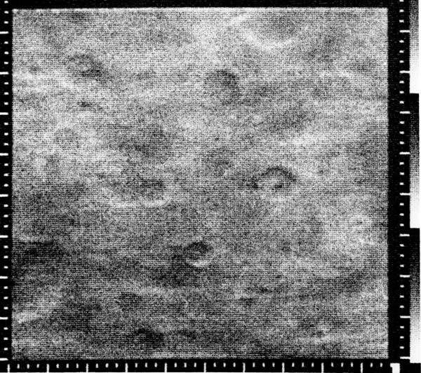
As examples of what might be considered sufficient data, consider some of the first historic missions that imaged the Moon and Mars, such as Luna 3 (first mission to image the Lunar far side) and Mariner 4 (first Mars flyby) both of which returned roughly 8 Megabits of data (1 MB). Here are examples of images from those first flyby missions.

7.3. Timing

Fig. 6. “First Image” Examples from History Estimated to be equivalent to 8 Megabits (1 MB) each

Wa = aV ΔV aD Dr − Do

) aTTot aI IV

(

Millis 2018 Grant NNX17AE81G_for_CR.docx

pg 35 of 69

Eq. 2

Extending the analogy to a possible orbiter mission, consider the Mariner 9 mission, the first Mars orbiter. That mission produced roughly 16 Gigabits (2 GB) of data. While these data quantities are small compared to recent planetary probes, such as Cassini-Huygens at over 600 GB, that was a Saturn probe at only about 10 AU from Earth. That’s 27 thousand times closer to Earth with communication that much easier. For our first interstellar missions, what are the lower bounds of what would be acceptable images? For example, a single image of an exoplanet in 6 bit gray scale, with 30 pixels across the equator (which would represent a tremendous leap beyond anything currently possible with astronomy) is about 4200 bits (0.5 kB).

Data Fidelity, If (?): Perhaps an additional factor could be how much is learned from a given volume of data,

though how to quantify such a parameter is uncertain.

Mission Ambition,” Wa (#): Finally, these factors combine to give a relative score for Mission Ambition. Since the individual terms use different units, normalizing and weighting coefficients, a, must be included for each term. A tentative equation for Mission Ambition is:

where higher interest is proportional to more time on target, higher data return, useful science at more distant instrument ranges, and more capable propulsion systems denoted by higher ΔV capabilities. Note that if the closest approach, Do, is greater than the instrument range, Dr, then the score for Mission Ambition goes negative. In other words, if the spacecraft cannot get close enough to the destination for the science instruments to do their job, then the mission is a failure. Additional variations of Mission Ambition can be considered in developing an optimized metric.

€

The next question is about the duration of the mission, or more broadly the entire project. Since this study includes the research that predates the mission, those stages are also measured. Many stages have trades. The stages are:

pg 36 of 69

Total Project Duration, Ttp (yrs): This term means the entire span encompassing all the other stages, from the

point the research begins until receiving all of the data back from the probe.

Technology Maturation Duration, Trl (yrs): This is the time between the start of the research and when that research has advanced to approximately TRL-6, or advanced enough to allow planning and developing a mission. The trade here is whether to select less capable but more near term technology that will be ready sooner, or more capable technology that might be available later. This is related to the Incessant Obsolescence Postulate, which is mostly affected by subjective mission motives.

In the case of the “Precursor Era” missions, sufficient technology maturation exists to initiate trade studies, albeit the best projected performance can only reach 1,000 AU in 50 years with a 38 kg payload [32]. In the case of both the “Infrastructure Era” and “Breakthrough Era,” the Technology Maturation Durations have not yet been estimated.

Devising a means to estimate the durations of technology maturation and mission development are part of the goals of this Stage I study. These details are discussed in Section 8.5 “Estimating Comparative Rates of Advancement.”

Mission Development Duration, Tdev (yrs): This is the time between the beginning of the mission trades studies and the launch of the mission. It will likely be different for each of the three interstellar eras and therefore estimated differently. The trade here is to use less complex systems that can be built faster, or more capable systems to launch later. Again, this is related to the Incessant Obsolescence Postulate, but this time the duration is also a function of how soon the infrastructure will be available.

For the precursor era missions, this duration will likely fall within the 6-12 year span of the development of the

New Horizons missions and Cassini-Huygens, respectively.

In the case of mission architectures of the infrastructure era, this is dominated by the time for using the presumed preexisting infrastructure to build the spacecraft and any supporting new infrastructure (such as laser systems). Accordingly and per the methods in Section 8.3 “Measuring Infrastructure Dependence,” these following two development times will be estimated:

Spacecraft Build Duration, Tscb (yrs): This is the time it takes to build the spacecraft and fully load it with propellant using the infrastructure available at the time. Base Hardware Build Duration, Tbd (yrs): This is the time it takes to build any of the supporting propulsion infrastructure such as anything that needs to beam energy or reaction mass to the vehicle.

Total Mission Duration, Tm (yrs): The time between launch and receiving all of the data back from the probe.

It is the sum of these sub-stages:

Trip Time, Tt (yrs): The time between launch and arrival at the destination. This is a function of the payload mass, the energy available for propulsion, and the performance of the power and propulsion system. Signal Time, Ts (yrs): The lightspeed signal return time, a simple function of the destination distance and lightspeed. Data Transmission Time, Tx (yrs): The time it takes to transmit the full suite of the data back to Earth. This is a function of the communication system, its power, and apertures (both on the spacecraft and the receivers on Earth), where in principle smaller payloads with less power will have lower data rates and hence longer transmission times.

The demarcation points between these times are defined as: Research Commitment Year, Yrc (calendar year, cy): This is the calendar year when the commitment is made to begin advancing the required technologies up through TRL-6, initiating the development of the spacecraft and base hardware. Technology maturation is initiated at the start of the Research Commitment Year and extends to the Mission Commitment Year.

Mission Commitment Year, Ym (cy): The calendar year when the commitment to developing the mission is made. The required technology must be mature enough for reliable trade studies at this point, specifically TRL ≥ 6. Currently only the Precursor Era missions satisfy that condition. Mission development begins at the start of the Mission Commitment Year and extends to the Launch Year.

Launch Year, Yl (cy): The launch date is often cited as a primary mission goal, but the decisions needed to meet that goal are made years earlier. The challenge in developing the analysis is that sometimes this will be an

Millis 2018 Grant NNX17AE81G_for_CR.docx

input value, and sometimes a calculated value, depending on what are set as the driving parameters. The launch year follows the start of the Research Commitment Year and encompasses the sum of Technology Maturation Duration and Mission Development Duration.

Arrival Year, Ya (cy): This is the year the spacecraft reaches the destination, or more specifically, when its scientific instruments are within functional range of the target—able to begin acquiring and transmitting data back to Earth.

First Data Arrival Year, Yd (cy): This is when the first data arrives at Earth, thus confirming that the

spacecraft has arrived and is still functioning.

Mission End Year, Ye (cy): This is the point when all data from the probe has been received on Earth.

The final facet of starting a mission is the basic question, “Why?” Of all the facets of an interstellar mission, this facet is seldom examined. In the prior literature, the motives were often implicit, but with the implication that first arrival was the main purpose. Accordingly, there was often discussion about what is now called the Incessant Obsolescence Postulate, (that a newer probe will pass the older, so why launch yet?) and how that was an impediment to progress toward interstellar research. The postulate favors waiting until the technology has reached some peak performance before committing to a mission (such as possible mission durations of less than 30 years). However, this posture is only valid if the motivation is to reach the destination first.

There are many other motivations for an interstellar mission other than the bravado of being the first to the goal line. Another motivation is the survival of humanity, where the relevant technologies of sustainable habitats would have value on Earth long before any interstellar world ships would be possible. Another motivation is technology development, of launching missions for the goal of testing the technology and testing the environment through which future probes will follow. A closely related motive is commercial endeavors, where the technology developed under the theme of interstellar flight would have nearer-term commercial applications. Perhaps this is a significant motive for StarShot, where powerful lasers and further miniaturized spacecraft have marketable potential, even if the technology never reaches the levels for enabling an interstellar mission. And last, but certainly not least, are the motives of science and curiosity—finding out what is really out there.

Sum of Motives, Wm (#): This variable is introduced to bring this often implicit and overlooked motivation factor into the discussion. In principle, for any given interstellar mission, that mission would be considered more valuable, and hence fundable, if it satisfies multiple ambitions and multiple stakeholders: NASA, commercial space, science, national security, global security, and general public interest. To provoke discussion on those relative motives, table 9 lists a number of motives, the consequential emphasis of each, and a subjective provisional value score. These provisional scores are based on Maslow’s hierarchy of human needs (survival, security, belonging, self- actualization). Sum of Motives is calculated simply as the sum of importance scores for each motivation that the mission addresses.

Table 9. Span of Motivations, Consequences, and Provisional Rankings

7.4. Motive

Scientific curiosity

Motivation

Sustainable habitats
Commercial utility (ROI)
Learn by doing
Maturing technology to readiness
Pursuing propulsion and power research that
First to launch or arrive
First to exceed some milestone

Consequential Technology Focus

are beyond marketable fruition

Instrumentation

pg 37 of 69

What, ultimately, is most important to mission planners? Presumably, it’s having an interesting enough mission that will appeal to a number of stakeholders and be accomplishable within a reasonable time and expense. To make

Millis 2018 Grant NNX17AE81G_for_CR.docx

Survival of humanity Technology development

Bragging rights (being first)

7.5. Figures of Merit

Subjective (provisional) Importance Score

these explicit and measurable so that mission and propulsion options can be compared, the following variables are introduced:

Mission Composite Value, W (#): The value of a mission is defined here as a function of the interest in the destination, the number of motives answered by the mission, and the fidelity of the data that the mission will collect. In principle, this is envisioned as a weighted sum of the “Destination Interest,” Di, “Mission Ambition,” Wa, and “Sum of Motivations,” Wm. The higher the value, the better.

Total Mission Expense, Etm, (J): This is a measure of the resources required to build, launch, and operate the mission. Instead of using financial cost, whose estimations require subjective predictions, the measure will be in terms of the energy, a fundamental, calculable physics parameter shared by all methods. The energy to “build” the mission will be in terms of the required infrastructure, while the energy to launch the mission will be in terms of propulsion energy. Since the expense of operating the mission after launch is assumed to be much smaller than the other factors, it will not be quantified. Specifically, then, “Total Mission Expense,” Etm, (J) is the sum of “Total Infrastructure Energy,” Eti, (J) and “Total Propulsion Energy,” Etp, (J). The lower the value, the better.

Total Project Duration, Ttp, (yr): As mentioned previously, this is a measure of how much time remains

between now and the point where all the data has been transmitted back to Earth. The lower the value, the better.

Mission Efficiency, We, (%): The final figure of merit is the efficiency of the mission, which is defined here as the ratio of the kinetic energy imparted to just the payload, Epy, and the Total Mission Expense, Etm. The higher the value, the better

An alternative definition of Mission Efficiency could be in terms of the Data Volume, Iv, and perhaps Data Fidelity, If, delivered per Total Mission Expense, Etm. In that case, the prior definition of Epy/Etm could be called “Vehicle Efficiency.”

It is anticipated that the Stage II and III analyses will reveal which of these factors are more or less impactive of

the technology requirements. Thereafter, choosing the relative importance of the options can be informed choice.

pg 38 of 69

Millis 2018 Grant NNX17AE81G_for_CR.docx

The major difference between the first two eras is the degree of infrastructure needed to support the mission. The distinction of the third era is that it requires further advances in physics (whose infrastructure needs are temporarily unknown). Comparisons within these eras are more easily achieved than comparisons across these eras.

8.1.1. Era of Precursors

This era refers to missions that can be launched from Earth with foreseeable technology and without needing substantial new infrastructure. By “foreseeable technology” it is meant those technologies that are already at, or above TRL-6. Examples in this era include:

METHODS FOR EQUITABLE COMPARISONS

Tied to the mission choices, it is necessary to measure the associated propulsion performance and the expense to deliver that level of performance. To make these calculations equitable across differing missions and differing propulsion methods, the basic strategies are: 1) start with comparing technologies that are at comparable readiness levels before advancing to compare across significantly different readiness levels 2) compare different propulsion and power concepts using common payload and mission scenarios, 3) devise a common means to measure the expense of building the mission hardware, 4) measure the performance of the disparate propulsion and power approaches using fundamentally common units, and finally 5) devising methods to compare technologies that are at different readiness levels and advancing at different rates.

8.1. Distinct Eras of Interstellar Flight

A starting point is to separate concepts that are at substantially different readiness levels. After reviewing the span of mission concepts and technology prospects, they can be divided into these distinct eras of interstellar flight:

Era of Precursors
Era of Infrastructure
Era of Breakthroughs

Voyager
Heliopause Interstellar Probe concept of 1999 [22, 24, 25]

Innovative Interstellar Explorer concept of 2006 [23] * Interstellar Medium Mission concepts 2015… [29, 31]

Project Daedalus, 1978 [49]
Forward’s Microwave Staged Lightsails, 1984 [48]
Project Icarus (started 2009) [79]
Breakthrough StarShot, 2016 [7, 40, 57-62]

Millis 2018 Grant NNX17AE81G_for_CR.docx

pg 39 of 69

For assessment purposes, the performance projections of those technologies are accurate enough to proceed to mission trade studies. Thus, they are not subject to the assessment methods of this report. These concepts are however used as baselines and scaling examples in this study.

8.1.2. Era of Infrastructure

The era of infrastructure refers to propulsion and power concepts that are rooted in the established laws of physics and are a matter of further engineering. This is where the bulk of interstellar propulsion concepts reside. The reason this is called the era of infrastructure is because even the smallest payload example from this group (1 g) requires substantial new infrastructure, specifically a 100 GW laser array spanning 1 square km. Examples of concepts in this era include:

The performance projections of these concepts are ambitious and still unproven, making the use of traditional trade studies unreliable. The other unknown for each concept is the remaining time required to mature its suite of

pg 40 of 69

technologies to mission readiness. And lastly, these concepts assume that the required infrastructure already exists— but there are no roadmaps yet to develop that infrastructure. The process for estimating the dependency of the mission architectures on infrastructure is explained in Section 8.3.

8.1.3. Era of Breakthroughs

The era of breakthroughs refers to concepts aimed at the highest impact, revolutionary performance gains that go beyond extrapolation of existing technology. This requires further advances in physics. A starting reference for the span of these concepts and the next-step research required to further assess them, is the book, Frontiers of Propulsion Science [13]. Examples of concepts in this era include:

Negative mass propulsion, 1957 [80, 81]
Propellantless thrust via inertial fluctuations (1994), now called “Mach Effect Thruster” [82-86]
Spacedrives, in general [87]
Dynamical Casimir Effect, 2004 [88]
Traversable wormholes, 1988 [11, 13 ch.15]
Warp drive, 1994 [12, 13 ch.15 ]
Faster than light communication [13 ch.16, 89-91]

In addition to propulsion and power breakthroughs, breakthroughs in communication can also play a powerful role in enhancing the mission—especially considering the impact on total mission duration. If FTL communication was possible, then the mission duration would be shortened up to a year for each light-year distance. The possibilities of FTL communication are discussed in the literature, including some quantum and other communication systems [89-91].

For assessment purposes, some of the breakthrough concepts have matured to the point where their propulsive energy can be calculated. For others, hypothetical analogs will need to be specified. In the case of generic spacedrives, for example, the propulsive energy can be modeled with basic kinetic energy and an efficiency factor for energy conversion. Section 8.4.4 describes the initial attempts for making estimates of this group.

Regarding their infrastructure dependence, this cannot be accurately determined until after they have been

sufficiently advanced to TRL 3.

8.2. Baseline Mission & Payload Scenarios

To compare different propulsion and power methods equitably, the same payload and mission scenarios are employed. To begin this process, five test-case mission and payload scenarios are envisioned. These scenarios do not need to accurately match an actual mission, but are close representations to allow comparisons of the different technologies.

One of the seldom specified details of proposed interstellar mission architectures is how much data will be returned and at what rate. Without specifying the amount of data to return, it is not possible, even in principle, to compare different mission architectures with different data rates. That is why the payload specifications are fixed with these mission scenarios. For the first four scenarios, the baseline payload is 100 kg, which is roughly based on a 200 W communication system intended to transmit 8 Megabits of data (1 MB) and assuming contemporary technology. Though this is a small amount of data, it is a minimum threshold comparable to the first historic flybys of the Moon and Mars (Luna 3 and Mariner 4, respectively) shown in figure 6 in Section 7.2.2.2. For the orbiting scenario, the payload and data quantity are increased. The payload for an orbiter is 1,000 kg, with a data about of 16 Gigabits (2 GB), analogous to the first Mars orbiter, Mariner 9.

Solar Gravitational Lens, > 660 AU (0.1 x 1015 m, 0.01 ly)
Deep Interstellar Medium, > 27,000 AU (4.1 x 1015 m, 0.43 ly)
Centauri Flyby, > 270,000 AU (41 x 1015 m, 4.3 ly)
Centauri Slower Flyby, > 270,000 AU (41 x 1015 m, 4.3 ly)
Centauri Orbiter, = 270,000 AU (41 x 1015 m, 4.3 ly)

Millis 2018 Grant NNX17AE81G_for_CR.docx

that the assessment methods function as intended.

8.2.1. Solar Gravitational Lens

Plots of the data for the first three of these missions are provided in Section 9, using different hypothetical

technology examples spanning the propulsion types described in Section 8.4.

In the final analysis system, individual mission choices can be specified. These initial examples are to verify

This mission in analogous the “FOCAL” missions of Claudio Maccone [36], and the more recent “Solar Gravitational Lens” mission of Slava Turyshev [37]. It involves sending an imaging payload out past 550 AU where focal length of the gravitational lensing of our Sun begins to appear (and continues outward). Using the magnifying effect it has been estimated that an exoplanet on the opposite of the Sun could be imaged to 10 km scale resolution.

There is also the possibility that the lensing effect can serve as a communications relay experiment for long- range microwave communication or optical communications relay for a high-data rate interstellar missions, and hence change the power requirements for a specified data rate. The reason this scenario is used is because it represents an actual purposeful location that is close to the threshold of what could be reached with precursor era technology. In other words, it is probably the first step to future, full-fledged interstellar missions.

8.2.2. Deep Interstellar Medium

In the vast void between the gravitational lens location all the way to the Centauri stars, there exist only sparse densities of comets and asteroids; the Hills cloud (2,000 AU), Oort cloud (10,000 AU), and the G-cloud (41,000 AU) [38]. Or in other words, it is the next easiest destination short of the big jump to Centauri. These features are difficult to discern using Earth-based astronomy, yet probes could make direct in-situ measurements. Consider a cloud sampler (particle and fields data, dust counters, radiation detectors) and discover how those values differ in different regions. Again a 100 kg payload mass and 200 W for communication is baselined.

8.2.3. Centauri Flyby

For the first flyby missions of an exoplanet, the analogy used to determine a minimum threshold of data is the first flybys of the Moon and Mars, specifically Luna 3 and Mariner 4, respectively. (see figure 6 in Section 7.2.2). The total quantity of data for each of these was roughly 8 megabits (1 MB). While this lowest threshold might seem too low, consider that Luna 3 showed enough to determine that the far side of the Moon was different than the front, and Mariner 4 showed that Mars was not like Earth.

pg 41 of 69

To broaden the trade space, the more challenging and rewarding trajectory of entering orbit is included. In principle, the ∆v of this mission is roughly twice that of flyby missions. The premise is that the spacecraft would have a telescope that could find all the “planet-sized” bodies in the system while approaching the system, and then have the ability to maneuver into an orbit around a target of interest (ideally perhaps with a flyby or two along the way of other bodies). Thereafter the spacecraft can observe long enough to see seasons, weather, imaging of the planet, solar wind and stellar activity, and send back this kind of data. For this scenario, the baseline payload and data quantity are increased. The payload is now 1,000 kg, with a data about of 16 Gigabits (2 GB), analogous to the first Mars orbiter, Mariner 9.

Ideally, propulsion for such maneuvers should be free of any dependence on propellant or beamed energy. They could either use onboard power or energy harvested as the spacecraft approaches the star system. If there is an ample stellar wind from the target star, then sail concepts like magnetic, plasma magnet, and electric could be considered.

This is also the kind of maneuver where the spacedrives of breakthrough propulsion physics apply. Or to rephrase; the ability to decelerate upon reaching the mission target, or more generally to maneuver without dependence on propellant or energy beamed from Earth, is a goal for which breakthroughs are sought. If the Mach

8.2.4. Centauri Slower Flyby

8.2.5. Centauri Orbiter

This scenario has the same payload and data requirements of the simple flyby, but this scenario is introduced to

consider the added value and expense of slowing down for the flyby.

Millis 2018 Grant NNX17AE81G_for_CR.docx

pg 42 of 69

Effect Thruster, now under test, is found to be both feasible and scalable, then one of its higher-performing successors might make these double-delta-v missions achievable.

8.3. Measuring Infrastructure Dependence

This study includes the use of infrastructure as part of the total mission. For two concepts whose performance is otherwise equal, the one requiring less infrastructure is preferred. Consider the classic interstellar concepts like Daedalus or Forward’s microwave sails which assumed the preexistence of a substantial in-space infrastructure. Which of those divergent approaches would require less time and energy to build, assuming all other factors were equal? For example: will it be easier to mine He3 from the atmospheres of the gas giants to support fusion propulsion, create a dedicated antimatter factory to support antimatter rockets, or to build TW lasers and 1000 km diameter Fresnel lenses? And in the course of answering those questions, which requisite technologies might be revealed to be more crucial or broadly applicable?

Recall the distinction between the era of precursors and the era of infrastructure. In the strictest sense, the era of precursors use established ground-based infrastructure and propulsion methods that are mature enough to proceed to trade studies. Hence those dependencies are not measured here. For true interstellar missions, however—the ones reaching to the nearest starts—new infrastructure is required. Regarding the era of breakthroughs, those concepts will fall into either the precursor or infrastructure era, on a case-by-case basis, depending on the scale of mass and energy required. Those concepts might need to be advanced to TRL 3 before such a determination can be rendered.

There is a split in the era of infrastructure concepts; those concepts that involve power beaming from the surface of the Earth (like StarShot), and those concepts that assume the use of preexisting in-space infrastructure (like Daedalus and Starwisp). These require two different assessment methods.

The fundamental units for comparing infrastructure dependence are mass, energy, and time. In principle, larger and more massive spacecraft will require more time and energy to build. The same is true for the systems that beam energy to the spacecraft.

For the ground based infrastructure systems, only the energy to build the beam system is measured, not mass nor the time to build that beam. This is because Earth-based construction will likely be considerably faster than in- space construction. For the in-space systems, both energy and time are measured. For the in-space scenarios, two factors need to be assessed, 1) predicting what infrastructure will be available for use over the future years, and 2) then estimating how much of that infrastructure is used to support the development of the mission.

These analyses are more relative than deterministic. In other words, the assessment can distinguish which mission plans will require more or less infrastructure, but will not be able to accurately predict how much time and energy that process will require.

One further note: It is reasonable to consider that the same kind of laser array considered for propulsion might also be the primary source of power delivery for the entire infrastructure. The assessment methods to include that possibility have not yet been established.

8.3.1. Earth-Based Beaming Infrastructure

For those concepts which aim for true interstellar distances (≥ 270,000 AU) and that assume their beaming infrastructure resides on the surface of the Earth, it is already possible to compare those systems against each other in terms of financial cost, instead of the more general measure of energy used throughout this study. To compare these concepts in energy terms, a conversion factor of $0.06/kW-hour, or 60 MJ/ $w i l l b e u se d . T h eeco n o mi c t h eor y b e hin d t hi sco n v er s i o n [92] w o u l d b e a l e n g t h y d i sc u ss i o n . P u t s im pl y, b ec a u see n er g y i ss u c ha f u n d am e n t a l in p u tt o a l m os t e v er y t hin g e l se ma d e an d u se d in c i v i l i z a t i o n, t h e " r e a l " cos t o f e n er g y (in t er m so f h o w man y g oo d s an d ser v i ces a^{'} u ni t o f e n er g y^{'} b u y s) c han g es v er y s l o w l y w i t h t im e . S ma l l er r or s in t h e f i g u r ec h ose na s a co n v er s i o n f a c t or i s n o t v er y ser i o u s in t er m so f co m p a r in g p r o p u l s i o n sy s t e m s, so l o n g a s i t i s u se d co n s i s t e n tl y . T h ees t ima t es f or c a p i t a l cos t o f a g i v e nb e am c an t h e nb eco n v er t e d t oe n er g y t er m s u s in g t ha t co n v er s i o n f a c t or . I f in v e n t i o n sc han g e t h ec a p i t a l cos t o f a g i v e n t y p eo f b e am (l o w er$ /Watt), then that is essentially equivalent to improving the “propulsion efficiency” of that type of beam, in that the lower $/Watt of beam power shows up in the comparison charts as a lower “total energy” (because of the reduced capital cost of the installation, expressed in energy terms).

It is conceivable that some Earth-based infrastructure might also have in-space components (hybrid concepts such as ground based optical beams with space-based focusing optics, or space-based particle beams with their

Millis 2018 Grant NNX17AE81G_for_CR.docx

power fed from the ground, are possible). The cost to create these new elements can be estimated by the launch costs ($/kg, J/kg) required to get that hardware into its orbital position.

8.3.2. Estimating In-Space Infrastructure Availability and Growth

For the more general suite of interstellar concepts that presume the existence of in-space infrastructure, the two major questions are” “When will the needed infrastructure be ready to support the mission?” and “How much will it cost in energy and time to use that infrastructure to build and launch the mission hardware?”

Currently, there are no substantive predictions about in-space infrastructure capacity and growth. As a starting point, the author sought the opinions from a number of subject matter experts (discussions with Brandt, Lewis, and Lubin, and cited values from Hoffman, Klupar) and merged them together to produce table 10 (with subjective compromises for mismatched predictions). Note how many fields remain unspecified. The rest of this table will be populated with estimates in Stage II of this work.

To get a grounding reference to scale the situation, the growth of world energy production has been extrapolated to fill out the first row in table 10. The data behind those extrapolations span 1888 through 2017 [46-47]. In the second row those values are converted into equivalent power (J/yr into J/s=W). The third row contains estimates from subject matter experts.

Since these projections will be used for relative comparisons only, it is not necessary that these growth projections be accurate. They only need set an approximate scale and then have that scale used consistently throughout the rest of the analyses.

Table 10. In-Space Infrastructure Availability and Growth Estimates

2020 2030 2040 2050 2060 2070 2080 2090 2100 2110

Functionalities:

Mining

infrastructure functions:

5.3 x

6.4 x

5.3 x

9.1 x 7.6 x

1020 5.3 x 5.3 x

1013 1 x 108 2 x 109 1 x

1.0 x

5.3 x

1.2 x

5.3 x

105

REFERENCE POINT: World Energy Production Extrapolation, (J/yr) REF: World Equivalent Power Capacity, (W)

Predicted Infrastructure Available Power, (W)

Capacity (kg/yr) Specific Energy (J/kg)

Material Processing Capacity (kg/yr) Specific Energy (J/kg) Manufacturing & Construction

Capacity (kg/yr) Specific Energy (J/kg) Connecting Transportation

Capacity (kg/yr) Specific Energy (J/kg)

Mining raw materials (including propellants)
Processing the raw materials into usable stock [100 MJ/kg aluminum?]
Manufacturing components from stock
Constructing objects from components and stock
Transporting items within the infrastructure

1.7 x

5.3 x

2.3 x

5.3 x

2.0 x

5.3 x

3 x

pg 43 of 69

Infrastructure Use Specific Energy, Esi (J/kg): For the analyses that follow, the specific energies for each of those functions will need to be estimated during stage-II. The sum of those specific energies will then represents the

The lower rows of table 10 refer to both the capacities (kg/yr) and specific energies (J/kg) of the various

Millis 2018 Grant NNX17AE81G_for_CR.docx

1.5 x

5.3 x

total Infrastructure Use Specific Energy, Esi, to be used when calculating the use of infrastructure. It is assumed that theses values might change over the decades of progress.

Infrastructure Available Power, Pia (W): The other key descriptor for the infrastructure will be Infrastructure Available Power, Pia, whose values will significantly change over the decades of progress, as provisionally indicated in the 3rd row of table 10. That factor will be used to determine how quickly the infrastructure energy can be expended, to estimate how long it takes to build things in space. Ideally, it would be more accurate to create a measure of infrastructure capacity, (kg/yr), from the estimates for the capacity for each of those functions. In the absence of that more detailed information, however, the more basic measure of Infrastructure Available Power, Pia (W), will have to be estimated as used for estimating how quickly things can be built with the infrastructure. Note that the only estimates obtained so far for capacity are for mining (kg/yr) for the 2030 and 2040 decades.

8.3.3. Estimating In-Space Infrastructure Usage

In principle, larger and more massive spacecraft will require more time and energy to build. The same is true for any beaming system for the mission. Thus, the first step of assessing infrastructure dependence requires knowing the total mass of the spacecraft and any supporting launch (beaming) hardware (whose calculations are described in Section 8.4):

Spacecraft Launch Mass, Msl, (kg)
Base Hardware Mass, Mb, (kg)

Spacecraft Hardware Build Energy, Esc (J): This is the measure of how much energy is required from the infrastructure to build the spacecraft. It is the product of the Spacecraft Launch Mass, Msl, (kg) and Infrastructure Use Specific Energy, Esi, (J/kg).

Base Hardware Build Energy, Eb (J): This is the measure of how much energy is required from the infrastructure to build the base hardware. It is the product of the Base Hardware Mass, Mb, (kg) and Infrastructure Use Specific Energy, Esi, (J/kg).

Total Infrastructure Energy Expense, Eti, (J): This is the sum of both the spacecraft and base hardware build energies, representing the total amount of energy needed to prepare the mission. The propulsive energy to perform the mission is discussed in Section 8.4.

The next question is: “how long will it take to build those objects?” The crude model used as a starting point is to divide the Build Energies by the Infrastructure’s Available Power, Pia, (W), and convert the answer from seconds to years, whose sum is the variable named Mission Development Duration, Tdev (yrs).

Spacecraft Build (develop) Duration, Tscd (yr): This is the measure of how long it will take to build the spacecraft, calculated by dividing the Spacecraft Hardware Build Energy, Esc, by the Infrastructure’s Available Power, Pia, (W), and convert the answer from seconds to years.

Base Hardware (develop) Duration, Tbd (yr): This is the measure of how long it will take to build the Base Hardware (like laser arrays), calculated by dividing the Base Hardware Build Energy, Esc, by the Infrastructure’s Available Power, Pia, (W), and convert the answer from seconds to years.

pg 44 of 69

Millis 2018 Grant NNX17AE81G_for_CR.docx

8.4. Measuring Disparate Propulsion & Power

This is part of the more deterministic portion of the analyses. The objective is to quantify the performance of each propulsion and power concept with respect to payload mass and total mission ∆V. The challenge is that the propulsion concepts are significantly different, each with its own components and figures of merit. For example, rocket performance is described in terms of specific impulse and thrust. Laser-sail performance is described in terms of beam power, beam divergence, etc. To compare these disparate methods equitably, the strategy is to reduce each to the most fundamental physics measurements of energy, mass, time, and power. In essence, energy is the fundamental currency of all motion. Specifically, this requires converting their usual performance parameters into the following more basic measures that are used in other parts of the analysis:

Total Propulsion Energy, Etp (J)
Spacecraft Launch Mass, Msl (kg)
Base Hardware Mass, Mb (kg) (For in-space infrastructure)
Energy Cost of Beam, Ebhw ( $, co n v er t e d t o J u s in g a J /$ scaling factor, for Earth surface hardware)

From these measures, other figures of merit can be calculated. To accommodate the span of possibilities, four different analysis techniques have been developed to cover the range of the power and propulsion methods. The distinctions depend on if the concept’s power is received from an external source (R) or internally (I), and if their reaction mass is onboard (O) or external (X). The variables associated with each of these distinct assessments are listed in table 6, “List of Variables,” along with annotations of which variables apply to which group.

Propulsion Type Examples

Power Source Reaction Mass

RP-OM

RP-XM

IP-OM

IP-XM

Table 11. Power & Propulsion Analysis Types

Chemical Rocket Nuclear Rocket Solar Thermal Rocket Laser (or solar) Electric Propulsion Laser (or solar) Sail Particle Beam Plasma Magnetic Sail SpaceDrive

Received

Internal

Onboard

External

pg 45 of 69

At this stage, only some of the conversion methods have been outlined, with further refinements to occur in Stage II. Also, for this first introductory stage, the proposed equations are nonrelativistic. This is a reasonable initial assumption since relativistic changes do not become significant (> 1.0% change) until past 14% lightspeed. In Stage II the relativistic equations will be included.

It should be noted that this approach is not the only method for analyzing missions in more general terms. In particular there is the “method of equivalent lengths” for both “energy limited” (e.g., chemical, high-thrust systems) and “power limited” (e.g., low thrust ion propulsion) systems [93-97].

Another caveat is that this starting assessment assumes that the same propulsion method is used for the entire journey. Future refinements would include assessing the merit of different propulsion types at different stages of the mission. For example, consider the prospects of accelerating the craft first by laser, then later by rocket, and then braking perhaps with a magnetic sail. It has been postulated that rockets might make better second stages, while laser propulsion would make better first stages. This is because the laser performance decreases as the spacecraft increases speed, and the ∆V of a rocket is independent of its velocity at ignition. Further refinements are necessary to evaluate such trades.

8.4.1. Type IP-OM: Internal Power & Onboard Reaction Mass

This type refers to systems which carry their own energy supply and reaction mass, such as chemical rockets,

nuclear thermal rockets, nuclear-electric rockets, and antimatter rockets. For this case, there is no beam system.

Millis 2018 Grant NNX17AE81G_for_CR.docx

The key performance characteristics of concepts in this category, where the propellant is also the energy source,

A given propellant has its unique specific energy Esp (J/kg), and a given propulsion method has an overall thrust conversion efficiency η (the fraction of the energy in the propellant which appears in the exhaust stream power). Energy which is lost to space, turned in to waste heat for the cooling system, etc., does not appear propulsively and so only that portion of the energy which appears in the exhaust stream is suitable for computing exhaust velocity and subsequent parameters. The amount of waste heat has an important impact on the mass of the spacecraft system (radiators, for example), discussed later.

An overall propulsion system (defined here to include all the spacecraft masses except payload and propellant) has a unique Propulsion System Specific Power, Psp (W/kg), that can be expressed in terms of the jet power Pj (W), propellant mass flow rate, dm/dt (kg/s), thrust force, F (N), and effective exhaust velocity, Ve (m/s).

From this it follows that:

Energy in the Reaction Mass

can be distilled to these two parameters:

Propellant Specific Energy, Esp (J/kg)
Propulsion System Specific Power, Psp (W/kg)

Where

convenient.

(W/kg) is:

pg 46 of 69

€

⎛ ⎜ ⎝

F =

⎛ ⎜ ⎝

2 =

Pj =

dm dt

⎞ ⎟ Ve ⎠

⎞ ⎟ Espη ⎠

Ve = 2Espη

Pj M se

F M se

Psp =

Psp

a =

€

Eq. 4

Eq. 3

Eq. 5

Eq. 7

Eq. 6

For equitable comparisons, any design parameters used to calculate the masses of those subsystems should be identified. When comparing competing concepts that use common systems (tankage, radiators, etc.) they should all use the same design parameters. For example, concepts that use the same propellant should use the same tankage fraction (kg-tank/kg-propellant), and concepts which use the same radiator technology should use the same radiator specific masses (W/kg). The exception to this is when the competing systems that are based on different mission commitment years, Ym, where those design specs might have improved for the later model. Tracking how the design parameters might improve over the years is covered in Section 8.5.3.

Therefore, from this relation it can be seen that the Propulsion System Specific Power controls acceleration:

where the mass of the spacecraft (empty and without payload), Mse (kg) is defined to include:

Propellant storage
Engine
Nozzle
Radiators
Remaining spacecraft structure and elements (typically insignificant to those other masses)

€

So either the effective exhaust velocity, Ve (m/s), or propellant specific energy, Esp (J/kg) can be used, as

The relation between the mass of the spacecraft, Mse (kg), and the Propulsion System Specific Power, Psp

Millis 2018 Grant NNX17AE81G_for_CR.docx

For a flyby mission, the relationship between the total mission ∆V; acceleration (ave), ā; acceleration time, Ta;

acceleration distance, Da; coasting time, Tc; mission distance, Dd; and trip time, Tt; follow these relations:

The achievable change in velocity in free space, ∆V, comes from the familiar rocket equation (burnout form which assumes thrusting time is << trip time. Note: Chemical and nuclear rockets usually have very high thrust to weight {high Psp} and hence, the thrusting time is << trip time. This is not necessarily true for other systems.):

Acceleration can be integrated for changing mass ratio, and for relativistic cases, should be. An approximation used here is based on average acceleration. Average acceleration, ā, (if not artificially limited to reduce loads on the payload), is then simply thrust, F, divided by the spacecraft empty mass, payload mass, and half the mass of the propellant as shown:

€

= Empty Mass of Spacecraft associate with Propulsion System Specific Power (kg) = Mass of Payload (kg) € = Mass of Propellant expended (kg)

From these, the Spacecraft Launch Mass, Msl (kg)—a value used in other portions of the analysis—is:

And where: Mse Mpay Mp

€

a =

M p

⎞ ⎟ ⎟ ⎠

M se + M pay +

M sl = M se + M pay + M p

⎛ M se + M pay + M p ΔV = ln ⎜ ⎜ M se + M pay ⎝

2 Dd − Da ΔV

Tt = Ta +Tc

ΔV a

Da =

Ta =

Tc =

a Ta

Millis 2018 Grant NNX17AE81G_for_CR.docx

Eq. 9

Eq. 8

Eq. 10

pg 47 of 69

Eq. 11

Recall the other mission time parameter, Data Transmission Duration, Tx, discussed in Section 7.2.2, and 7.3. For orbiter missions, one must also account for braking time and braking energy, both of which can be significant. For that reason, orbiter missions often use a different propulsion method for braking. The extension from the above equations for type IP-OM systems is straightforward—half the delta-V available to accelerate, and half to brake. If another type of system is used, compute the braking time as appropriate for that system, and add it to the mission time.

€

Energy Separate From the Reaction Mass

This sub-category of IP-OM types refers to systems like nuclear electric propulsion, where a separate power source (e.g., nuclear reactor) supplies energy to a rocket to expel an inert propellant (e.g., Xenon ion thruster). These are usually treated in terms of specific power (kW/kg) or alpha (kg/kW), and specific impulse (or effective exhaust velocity).

However, in these cases, “propellant specific energy” doesn’t fit. One cannot turn the energy into thrust without the reaction mass (propellant). A general assumption can be made that one runs out of propellant before running out of energy. Therefore, treating the propellant capacity as the limiting factor, there may indeed be a meaningful specific energy to define. Still, in any given case, the achievable acceleration and ∆V are usually clear from the particular apparatus in question.

pg 48 of 69

€

8.4.2. Type RP-OM: Received Power & Onboard Reaction Mass

This type refers to systems which receive energy from external sources but carry their own reaction mass, such as solar-electric or solar-thermal rockets, or laser-illuminated electric or thermal rockets. The initial analysis provided here addresses the case of ground-based beam infrastructures which draw their power from the electrical grid. Their calculations for the propulsion energy also applies for the case of space-based infrastructure, but the additional cost to create that space-based hardware is explained in Section 8.3.3. Recall that the parameters that need to be calculated from the specifics of these types of propulsion include:

Total Propulsion Energy, Etp (J)
Spacecraft Launch Mass, Msl (kg)
Energy Cost of Beam, Ebhw ( $, co n v er t e d t o J u s in g a J /$ scaling factor)
Base Hardware Mass, Mb (kg) (For in-space infrastructure) [not yet addressed]

For The Spacecraft Portion

As these are still rockets, the equations of Section 8.4.1 still apply as far as computing trip time. However, now the jet velocity, Ve, is no longer determined by the energy intrinsic to the propellant as in type IP-OM, it is instead an adjustable parameter (within the limits defined by a given thruster technology; some thrusters have a narrow range of exhaust velocities, some a wide range). A given mission design therefore needs to specify the specific energy imparted to the reaction mass (alternatively, the exhaust velocity and thrust efficiency, which is equivalent, eq 5). In general, these systems are usually employed with total velocity change (∆V) which is comparable to or less than the exhaust velocity because the mass of power receptions and thrusters are often high enough to be incompatible with high mass ratios. Efforts to circumvent those limitations are ongoing.

The Propulsion System Specific Power Psp of these systems is usually dominated by the power supply, and affiliated systems, sometimes mistakenly neglected in naïve analyses, such as power conversion machinery and radiators for waste heat.

Furthermore, acceleration has to be analyzed in two phases: 1) when the beam or solar radiation fully illuminates the receiver at the limit of the power capacity of the spacecraft—in which case, it is the spacecraft which determines the attainable acceleration, and 2) when the spacecraft is too far to intercept full power of the beam, in which case the beam’s divergence causes available power to drop off with distance. A similar case exists for solar- electric propulsion, when the falloff of sunlight (1/r2) drops below the limit of the power capacity of the spacecraft.

For the Beam Portion

The process specified here is for ground-based beam systems, where the beam’s figures of merit are usually discussed as $/ w a tt o f b e am p o w er, an d$ /square meter of transmitter aperture. Thus the first generally relevant figure of merit for beams is:

Beam Source Cost Scaling =

Where “Beam Source” is the energy supplied to the beam, in terms of the beam’s output power.

Since beams are, very roughly, characterized by a certain cost per unit area of aperture, and twice the aperture radius gives half the divergence angle, but four times the area, that implies a beam with half the divergence angle has the “aperture contribution” to beam cost roughly four times higher.

€

Note that it is really the divergence angle of the beam that controls what the beam can do—different beams have different divergence properties that scale differently with aperture. Therefore, to define a figure of merit which is suitable for comparing both optical and particle beams, we want a figure of merit that is based on divergence angle. For optical beams, divergence angle is proportional to wavelength, and inversely proportional to the radius of the aperture. The beam director cost factor for an optical beam would be: Beam Director Cost ÷ Aperture Area, ($/m2).

But that doesn’t work for other types of beams, including synthetic sparse apertures and particle beams, especially beams that include a degree of self-focusing. Instead, the second generally relevant figure of merit for beams is defined here as:

Beam Director Cost Scaling = Divergence Angle radians

) × Beam Director Cost $( )

Cost of Beam Source $( ) Power of Beam Source W(

)

(

Eq. 12

Eq. 13

Millis 2018 Grant NNX17AE81G_for_CR.docx

Where “Beam Director” is the aperture-scaled hardware for focusing the beam. The utility of that rather odd

factor is clearer when put in terms of cost:

It is obvious that a smaller divergence angle (tighter beam), gives a higher cost. So the divergence angle has to be in the denominator. Because of the scaling being such that, very approximately, half the divergence angle tends to be four times (or more) the cost, not twice. Given those two factors for a given beam technology, other beams of higher or lower power, or smaller or larger divergence angle, can be roughly estimated.

8.4.3. Type RP-XM: Received Power & External Reaction Mass

This type refers to systems in which both the reaction mass and energy are supplied from external sources, such as solar sails, solar-wind magnetic sails, laser-pushed lightsails, and particle beam pushed magnetic sails. It also covers “pellet runway” concepts in which pellets, prepositioned ahead of the spacecraft, contain an energy source that the spacecraft uses to accelerate those pellets as a reaction mass (such as fusion-fuel pellets, e.g., Jordan Kare’s “Bussard Buzz Bomb,” an idea not published in journal form, but discussed in [98 p.112]).

While the details of each such system are quite different, and it takes some careful consideration of each system to fit it in to the overall comparison framework, they can be compared to each other, and to other systems, with the following approach.

As discussed in “Type RP-OM,” a given power transmitted by the beam, Pgb (W), and a given divergence angle, Θ (radians), is characterized by a beam source cost scaling factor ( $/ W) an d ab e am d i r ec t or cos t sc a l in g f a c t or (r a d ian s / s q r t$ ). A given beam also has a given speed of the energy transmission, Vb (m/s), which is the speed of light for photons and less for particle beams. For particle systems, the speed of the beam can be varied during the mission which is a powerful tool for optimizing total energy used.

The beam in turn pushes on something, called here the “receiver”—which has a characteristic ‘Areal Density’ (that is, mass, per unit area of the receiver, kg/m2), and a ‘Flux Limit’ (the maximum power per unit area of the receiver, usually set by thermal limits of the materials, W/m2). When the receiver is saturated, operating at its power limit, we can define the now-familiar Propulsion System Specific Power Psp for this situation:

€

Cost ($) =

(

⎛ ⎜ ⎝

⎞ ⎟ ⎠

⎞ ⎟ ⎟ ⎟ ⎟ ⎟ ⎠

) Divergence Angle radians

⎛ Beam Director Cost Scaling radians ⎜ ⎜ ⎜ ⎜ ⎜ ⎝

) Receiver Areal Density kg/m2

Receiver Flux Limit W/m2

⎞ ⎟ Dbl ⎠

⎛ F ⎜ M sl ⎝

Psp =

(

)

Eq. 14

pg 49 of 69

Eq. 16

Eq. 15

As in more conventional forms of propulsion, the specific power in turn controls acceleration, while the beam is saturated. In the general case, however, there are usually two distinct phases of flight, 1) limited by the receiver, in which the receiver is saturated and taking all the power it can handle, and 2) limited by the transmitter, in which the receiver area (and mass) is determined not by power limitations, but by the divergence of the transmitting beam. For any given concept, it is usually clear how to handle these to develop overall trip times. However, the optimization of trip time for a given set of technology assumptions is not always straightforward. In order to be able to handle the variables, a concept should list both the areal density (kg/m2) and the flux limit (W/m2) of the receiver, because some calculations need the parameters broken out.

€

Acceleration (Thrust/Mass) is then integrated over time to get velocity change. While in a realistic situation, the thrust tapers off as the beam diverges and less and less power is intercepted by the receiver, the equations have the same form as if the beam simply had a finite range. For example, Lubin has determined that for photon sails, the maximum velocity change is 1.4x the velocity obtained if the beam were cut off when the sail no longer intercepts the full beam (Beam Range Limit, Dbl) [99]. Therefore, while there is a correction factor (of order less than two), the velocity gain becomes:

ΔV = Beam Range Limit Correction Factor × 2

Millis 2018 Grant NNX17AE81G_for_CR.docx

For relativistic spacecraft speeds, one must reduce the value of beam power due to Doppler shift of the

The power to generate that photon beam, Pgb (W), is simply:

The Beam Range Limit, Dbl, is determined by the divergence angle of the beam and the aperture of the

For Photon Beams: For non-relativistic spacecraft speeds, the thrust for a photon beam is simply the power transmitted by the beam,

Pbx (W), divided by lightspeed:

Msl = Spacecraft Launch Mass (= Payload + Spacecraft Empty Mass,) (kg) Dbl = Distance of Beam Range Limit (m)

Pgb = Power to generate the beam Pbx = Power transmitted by the beam ηB = Power efficiency of generating the beam

For Particle Beams: The nonrelativistic thrust for a particle beam is:

Where:

receiver.

incoming beam.

pg 50 of 69

Where:

€

F =

Pgb =

Pbx c

Pbx ηB

⎞ ( ⎟ Vb − Vs ⎠

dm dt ηB

⎞ ⎟ Vb ⎠

dm dt

Pgb =

⎛ ⎜ ⎝

F =

⎛ ⎜ ⎝

)

Where: = Power to generate the beam (W) Pgb dm/dt = Participle Beam Mass Flow Rate (kg/s) € = Particle Beam Velocity (m/s) Vb = Power efficiency of generating the beam (%) ηB

dm/dt = Participle Beam Mass Flow Rate (kg/s) Vb Vs

= Particle Beam Velocity (m/s) = Velocity of Spacecraft (m/s)

€

The power to generate that particle beam, Pgb (W), is:

Eq. 18

Eq. 17

Eq. 19

Eq. 20

The energy cost for the beam is then the sum of the energy actually used in generating the beam times the acceleration duration (beam on) (Pgb x Ta) and the “energy cost equivalent” of the beam and the beam director (discussed in Sections 8.3.1 and 8.4.2).

For a given mission concept, all these factors can be adjusted to optimize trip time and power for a given destination, so a single number does not really express the capabilities and one must explore how the system scales to destinations of different distances at different power levels, generating a set of contours. This is the plan for

Millis 2018 Grant NNX17AE81G_for_CR.docx

presenting the (deterministic) data for the concepts so they can be meaningfully compared (see Section 9 for sample plots).

The same physics discussed above applies to “sailbeam” concepts in which, rather than launching particles or photons to the spacecraft, we use a photon or particle beam to push some kind of “nano-craft” or “chipsat” or “smart pellet” which have some ability to correct their own trajectory and thus home-in on a traveling craft [100]. This approach allows the resulting “smart pellets” to be used as propulsive mass by a suitable receiver on an accelerating spacecraft. This effectively creates a divergence-free beam, allowing for much longer acceleration times and hence lower power levels, balanced against the potentially higher cost (converted to energy equivalent) of the pellets and the added mass of a shock-absorbing system on the spacecraft (since each ‘pellet’ imparts an impulse to the spacecraft that is large compared to a photon or elementary particle).

The last class of concept of type RP-XM is the “pellet runway” [98 p.112]. The physics of this approach is somewhat different—in a pellet runway, rather than shooting “smart pellets” at the spacecraft, the pellets are launched before the spacecraft, and the spacecraft “runs over” the pellets as it accelerates. While this is purely type RP-XM by the nomenclature, the analysis is a hybrid approach—the launching of the pellets (and the energy equivalent of that), is computed using the equations of this section. However, the pellets, containing both the energy and the reaction mass, require some modification of the ‘propeller equations’ discussed under type IP-XM in the following section. For the majority of the trajectory in which the speed at which the spacecraft encounters the pellets, Vip (m/s) is large compared to the increase in velocity provided by the ‘jet’, the thrust is controlled by the specific energy of the pellets, Esp, and their thrust conversion efficiency η (as with type IP-OM), and one can approximate the thrust as:

Where:

⎞ ⎟ ⎠

F ≈

⎛ ⎜ ⎝

dm dt

2 − Vip

⎞ ⎛ ⎟ 2Espη+Vip ⎜ ⎝ ⎠

8.4.4. Type IP-XM: Internal Power & External Reaction Mass

This type refers to systems which receive reaction mass from external sources but carry their own energy. This is analogous to aircraft engines, where air is the reaction mass, and the energy source is the fuel. In terms of interstellar flight, this includes, for example, Bussard ramjets that gather protons and accelerate them with the help of onboard energy [101], and spacedrives that convert some form of stored energy into propulsive motion (kinetic energy) using as-yet-unconfirmed physics [82-87].

This category also includes “drag devices” such as magnetic sails (magsails) or plasma magnet sails. These devices are possible solutions to the challenge of braking at the destination. Without braking, the flyby time is very short. See table 8 in Section 7.2.1 for examples. After a flight time of decades, a flyby time of just hours seems disproportionate and would limit the fidelity of observations.

Therefore, the problem is not only one of how to get up to speed, but how to get rid of the speed. Drag devices—devices that serve the same purpose in interstellar flight as do aerobrakes and parachutes in planetary exploration—in principle dissipate the kinetic energy of the spacecraft against something else (usually, the ionized gases in the interstellar medium).

Finally, there is a class of potential “plasma wave” drive concepts in which traveling waves are launched in to the interstellar medium at a velocity far below the speed of light, and the resulting reaction force propels the spacecraft [102]. These are usually low specific power (low thrust) drives but they use the surrounding medium as reaction mass. Such an ability is similar to the goal of a spacedrive, but using existing physics.

Millis 2018 Grant NNX17AE81G_for_CR.docx

Eq. 21

pg 51 of 69

dm/dt = Participle Beam Mass Flow Rate into the spacecraft (kg/s) Esp η

= Pellet Specific Energy, where the pellets are both a reaction mass and carry energy (J/kg) = Thrust conversion efficiency (%)

€

From this one can see that the mass flow required for a given thrust rises with the speed that the spacecraft encounters the pellets, until the power limit of the machinery that converts the pellets to thrust (a reaction chamber and nozzle) is reached. The beam cost in this approach is potentially much lower, because the pellet speeds can be much lower. However, the mission time is increased, because to the flight time must be added the time to pre- position the pellets; that factor limits the potential energy savings.

In the case of interacting with the interstellar medium, during the dominant part of the trajectory, the speed of the spacecraft through the media, Vsm, is much higher than the delta V that the thrusting effect can impart to a portion of that media, ∆Vt (Vsm >> ∆Vt). In that case, the power equation can be approximated by the much simpler form which illuminates the fundamental truth of all such propulsion—that the faster the spacecraft, the higher the power requirements:

Depending on the nature of the reaction mass, the analysis methods vary. For things like plasma, interstellar protons, or stellar wind, analogies to aircraft propellers can be used. For new breakthrough propulsion physics (devices that can be viewed as using inertial frames or the properties of spacetime as an effective reaction mass), then other techniques are suitable.

Plasma Reaction Mass:

For concepts that interact with plasmas or interstellar protons, the fundamentals of conservation of energy and momentum result in the ‘propeller equations’ familiar for propeller and air-breathing jet operation within an atmosphere can be used:

dm/dt = Mass Flow Rate of media through thruster (kg/s) Vsm = Velocity of spacecraft through media (m/s) ∆Vt = Delta V of media by thrusting effect (m/s)

€

Where:

And where:

pg 52 of 69

Where:

€

]

P =

⎛ ⎜ ⎝

F =

⎛ ⎜ ⎝

dm dt

− Vsm(

⎞ ⎟ ΔVt ⎠

⎞ [ ( ⎟ Vsm + ΔVt ⎠

P ≈ F × Vsm

F M sl

ΔV =

€

∆V = Change in velocity imparted to the spacecraft, (m/s) Msl = Spacecraft Launch Mass (= Payload + Spacecraft Empty Mass), (kg) Ta = Acceleration Duration (s)

€

Eq. 23

Eq. 22

Eq. 24

Eq. 25

This applies both to thrust and drag devices—however, while available power supplies tend to have low Psp and hence low accelerations, some drag devices offer high decelerations because they are dissipating power in to the interstellar plasma rather than consuming it. Drag devices may be power-limited (in which case they can be modeled as thrust devices), or they may have a constant “ballistic coefficient” like a parachute, in which case their drag varies with the square of the velocity through the medium, 𝑉sm.

In the case where Vsm is high, one also must check whether thrust, F, needs to be replaced by a “net thrust” or thrust minus drag. It may seem counterintuitive that one would be concerned with “drag” in the thin interstellar medium, but devices to collect reaction mass, almost by definition, have some way of interacting with the interstellar medium and so do offer drag. Neglecting this led to some early over-estimates of performance of some types of Bussard ramjets, for example. While the means of estimating drag is rather specific to the particular device in question, it is usually sufficient for comparison purposes to check if it is significant at the speeds in question (it often is not), and to account for it only in cases where this is not so.

For acceleration using plasma reaction, Propulsion System Specific Power (Psp) of these propulsion systems is still very important; usually this is dominated by the power supply carried with the spacecraft. Because Type IP-XM systems are not limited by their stored reaction mass, the energy content of the power supply is what ultimately controls the ∆V available.

Millis 2018 Grant NNX17AE81G_for_CR.docx

Spacetime & Inertial Frames as Effective Reaction Mass:

Concepts like negative mass propulsion, the Mach Effect Thruster, and the warp drive all face the challenge of an ambiguous reaction mass. Regardless of those specifics, the techniques to estimate their performance can be crudely estimated in terms of converting stored energy into kinetic energy of the spacecraft, with some conversion efficiency, η, and a Propulsion System Specific Power, Psp, (W/kg). Absent of better values, comparable efficiencies and specific powers from other concepts can be considered as a starting point.

For the special case of the warp drive, energy conversion equations exist [13 p.491, 103], but there are no

equations yet that remotely resemble Propulsion System Specific Power.

8.5. Estimating Comparative Rates of Advancement

The timescales for interstellar missions are comparable to prior technological revolutions (figure 3). Thus it is entirely possible that a revolutionary technology will emerge and surpass the performance of a more evolutionary technology already in development. But how does one predict if, and when, that might happen and what to do about it?

Recall that the objective of this study is not just to reveal which propulsion concepts might be the most advantageous (and under which circumstances), but also to identify the most impactive supporting technologies to guide the selection of a prudent portfolio of next-step research. This requires developing methods to estimate, not only the impact of a particular technology, but also estimate when that technology might be ready for mission commitment.

While it is not possible to predict the future, technology developments do follow patterns that can be used as a guide. First, there are the “Technology Readiness Levels (TRL),” that are both a way to assess the readiness of a given technology as well as identifying what further steps are needed to advance that technology to mission readiness. Second, there is the “S-curve” pattern to technological improvements and revolutions that suggest how to model that process [41]. Another source under consideration is the “Technology Forecasting and Readiness Assessment” methods of Darryl Web, et al [104].

There are at least two distinctly different rates of advancements to model: 1) where the performance values of mission-ready (TRL ≥ 6) technology improve over the years, and 2) where potential increases in performance levels advance up the TRL scales, from concept to mission readiness. That first type, advancing performance over time, pertains mostly to baseline technologies shared by the different propulsion of power concepts (such as payload miniaturization). That second type, the maturation of new performance abilities, pertains more to the propulsion and power concepts being assessed.

All of these assessments will be relative rather than absolute. In other words, the assessment will judge if one technology might reach fruition before another, but will not be able to accurately predict the actual time when either will reach fruition. The key here, is that all the competing methods are compared to the same standards.

Caveat: At this time, none of these predictive tools have been completed and tested. This is an area where much will be learned in the attempt, but predicting the future, even in relative terms, carries with it a great deal of uncertainty. Absent of any alternatives, however, these methods are at least a starting point.

8.5.1. Baseline Performance Trends

To equitably compare different propulsion and power concepts, it is necessary that the parameters that they share in common be set to the same, baseline values. As previously discussed, identical payload and ∆V requirements are imposed when comparing different propulsion concepts. In addition, this is extended here to include common subsystem technologies that are the same across different propulsion methods, such as thermal radiators, tankage fraction (for the same propellant-based systems), and energy density for systems using the same energy storage technology.

These baseline values, however, will change over the years. To compare the overall performance of missions begun in different years, the rates and limits of these trends will have to be modeled. For consistency with the definition of “Mission Commitment Year, Ym,” described in Section 7.3, the values estimated for each year shall be those that have reached TRL ≥ 6. Table 16 shows an example of how this tracking might begin. Note that the last column is labeled “physics limit.” Trends can hit a limit. Miniaturization will reach a point where the number of

pg 53 of 69

Millis 2018 Grant NNX17AE81G_for_CR.docx

8E+14 ? 1 g ?

Trends to Model Performance levels of TRL-6 technology Available Mission Energy (J/y) (see table 10.) Payload Mass (by Miniaturization) (kg/function) Shared Design Standards

Power Source Power Density (W/kg) Energy Storage Density (J/kg) Tankage Fraction (for a given propellant)

Radiator specific mass (kg/W) Etc.

molecules per function cannot be further reduced. An example of a real propulsion limit is the maximum theoretical Isp of hydrogen-oxygen rockets, which is 528.5 sec Isp, (based on 100% conversion of stored energy into kinetic energy and a propellant specific energy of 13.43 MJ/kg).

It is expected that these trends can be modeled by exponential equations or nested S-curves (Section 8.5.3). To guide those equations, data on the performance level changes over the years and any limits (to set asymptotes) is required.

Table 12. Tracking Advancement Trends of Common Technologies

pg 54 of 69

2020

6E+14 ?

0.5 kw/kg ?

5E+14 ? 30 kg ?

3.7% (STS ET)

Related to these are the advancement rates for infrastructure readiness. This was already discussed in Sections

7.3 and 8.3. and repeated here for contextual reference.

8.5.2. Technology Maturation Rates

New power and propulsion concepts that show promise for increased performance (such as higher Isp, higher thrust, or lower beam divergence) will have to advance up the “Technology Readiness Levels (TRL)” to the point of being ready for mission consideration (TRL ≥6). But how long will it take for the technology to advance through the technology readiness levels?

The Technology Readiness Levels are both a way to assess the readiness of a given technology as well as identifying what further steps are needed to advance that technology to mission readiness. A possible tactic is to use the TRLs as a proportional scale of advancement time, where the time to advance from TRL-n to TRL-n+1 and the time to advance from TRL-n+1 to TRL-n+2 follow similar ratios. Granted, there are significant variations that render this tactic inexact, but if used just for relative, rather than absolute, comparisons, then it is a fair starting point. A provisional proportionality of TRL advancement durations is presented in table 13.

Note that table 13 also lists “SRLs,” “Scientific Readiness Levels,” for the scientific advancement that precede new technology. The levels shown are adaptations from the “Applied Science Readiness Levels” outlined for the NASA Breakthrough Propulsion Physics project [13 p. 683].

For example, what if a concept is now at TRL-3, and we want to estimate how long before it reaches TRL-6. If the history of that concept shows that it took two years to go from TRL-1 to TRL-3, (for which the provisional duration increments are 1+2=3), then its TRL rate multiplier is 66%, (2 yrs actual)/(3 units). By multiplying that rate to the remaining seven duration increments gives an estimate that it will take four to five more years to reach TRL-6. To determine a representative set of these relative TRL durations, the histories of several comparable technologies will need to be examined, and then their results merged into a baseline set of TRL durations. The factors that need to be specified include the challenges of the technology itself and the history of resources devoted to the advancements. Again, these predicative models are only meant to be relative, not absolute. The key is that the difference concepts are compared with identical models.

From experience, the advocates for a particular technology tend to overestimate the readiness of their concept. To get more accurate readings on a technology’s actual readiness level, the US Air Force developed a “Technology Readiness Level (TRL) Calculator” that is accessible online [105].

…

Physics Limit none? ?

Millis 2018 Grant NNX17AE81G_for_CR.docx

Table 13. Technology Maturation Levels and Relative Durations Between Them

Description of Level

Comments

Considered here to be part of the Mission Development Duration “Valley of Death” Ready for mission trades studies and mission commitment

Experimental test devised for a new power or propulsion mechanism

If found viable, ascends to TRL-1

Basic principles observed and reported

From system prototype to flight proven

Technology concept and/or application formulated

Component and/or breadboard validated in laboratory

Level

SRL-6

SRL-7

TRL-1

TRL-2

TRL-3

TRL-4

TRL-5

TRL-6

TRL 7-9

Duration Unit

(indeterminate)

SRL-1

SRL-5

SRL-4

SRL-3

SRL-2

Hypothesis devised for a new power or propulsion mechanism

Component and/or breadboard validated in relevant environment

System/Subsystem model or prototype demonstrated in a relevant environment

Analytical and experimental critical function proof of concept

Problem statement devised to seek a new power or propulsion mechanism based on established effects

New effect observed and reported that is relevant to power or propulsion goals

Hypothesis devised for an effect relevant to power or propulsion

Problem statement devised for an effect relevant to power or propulsion

Experimental test devised for an effect relevant to power or propulsion

Millis 2018 Grant NNX17AE81G_for_CR.docx

pg 55 of 69

To create these estimates, it would be helpful to examine the histories of key parameters like those listed in table 12. In addition to plotting performance steps over time, it would be helpful to know the resources expended to attain each improvement.

There are more influences on advancement rate than just the ratio of TRL steps. If a concept does not have enough history (or inconsistent history or resources and commitment), then the following additional factors require consideration:

Level of available resources—where greater resources lead to faster progress
Operating power of concept—where lower power devices are easier (faster) to advance
Complexity of concept—where simpler devices are easier (faster) to advance
Relation to S-curve—where the rate of progress is fastest when midway between the performance level of

the first embodiment to the level of its upper physics limit

8.5.3. Modeling Technology Advancement Rates in General

Technological advancements follow recurring patterns. One of those patterns is the “S-curve” of technology

advancement as described by Foster [41].

The S-curve evolution, shown in figure 7, is typical of any successful technology. The pattern begins where the initial efforts produce little improvement until a breakthrough is reached. The breakthrough, at the lower knee of the curve, is where the technology has finally demonstrated its fidelity. After this point significant progress is made with Recurring S-Curve Pattern of Advancements ever-improved versions of the same concept. Eventually, however, the physical limits of the technology are reached and continued efforts result in little additional advancement. This upper plateau is “the point of diminishing returns.” To go beyond these limits a new alternative technology, with its own S-curve, must be created. Examples include how jet aircraft surpasses the speed limits of propeller aircraft, or how steam ships surpassed the performance of *  To surpass that method, a different method is sailing ships. Note, the horizontal axis is not time as expected, but rather the resources ($ and time) devoted to the research.

*  Each method follows a similar development curve,

That last item, the “S-curve,” is the subject of the next subsection.

pg 56 of 69

Next Method

Prior Method

Theoretical Limit

e c n a m r o f r e P

eventually reaching a limit.

created which has its own curve

Resources Figure 7. S-Curve Pattern of Technology Advancement Foster (1986) Innovation - The Attacker’s Advantage, 1986

Exponential Growth: Sometimes it appears that performance gains follow an exponential growth, such as “Moore’s law.” Moore’s law is the observation (and subsequent extrapolation) that the number of transistors in an integrated circuit double about every two years. While this trend might hold for a while, eventually a limit is reached. For example in the extreme, is it safe to assume that transistors can never get smaller than a single subatomic particle? Further, it has also been shown that these apparently exponential growths in performance are actually a sequence of overlaid technology “S-curve” advancements [106].

Changing Advancement Rates: Note from figure 7 that the rate of performance gains, verses resources applied, is the greatest when a given technology is at the midpoint of its development. As expected, early progress is slow. What is often overlooked with well established technologies (ones near the top of their S-curve) is that additional performance gains get increasingly more costly to obtain and reach a point where no further performance gains are possible. An example of this is the history of LH2 rocket engines, where its theoretical limit is 528.5 sec Isp, (based on 100% conversion of stored energy into kinetic energy and a propellant specific energy of 13.43 MJ/kg) and the Space Shuttle Main Engines achieved 452 sec Isp, after considerable investment.

Thus, when considering the rates of future advancement of a technology if using the TRL step analogy, then that rate will become slower for technological concepts that are approaching their upper theoretical operating limits.

Indicators for Emerging Breakthroughs: History has repeatedly shown that the conditions are ripe for breakthrough technologies to emerge when the following two conditions have been met: 1) The prior technology is reaching the point of diminishing returns, and 2) Clues have emerged for how to seek those breakthroughs (that it’s

There are multiple lessons that that go along with this recurring pattern:

The appearance of long-term exponential growth in performance is actually a series of S-curves
Advancement rates vary depending on how mature the concept
This pattern is mathematically describable by a “Logistic Function”

Indicators exist for when it is appropriate to seek new S-curves (“breakthroughs”)

Millis 2018 Grant NNX17AE81G_for_CR.docx

L = Upper asymptote, analogous to the physics limit of the concept k = Maximum rate of progress at the mid point of the concept’s development

y = A measure of performance of the concept (Isp, thrust, w/kg, etc.) where the y=0 point is

approximately the first demonstrated functionality of the device

x-x0 = Level of resources expended

not just science fiction any more). By “clues” it is meant that there are actionable and relevant research steps that can now be taken.

An arguable case in point is the emergence of the “Mach Effect Thruster” and other claims of propellantless propulsion. In this case the prior technology, rocketry, is at, or nearing, its point of diminishing returns. The degree of progress that can be gained for a given level of investment is far less now than in the early years of rocketry. The second criteria is the emergence of clues for alternatives. In this case, the correlation between the desired breakthrough of a propellantless thruster and specific unexplored topics of physics were identified and published spanning the mid-1990s through 2010 [13]. One of the relevant open questions in physics regards the origins and structure of inertial frames—clues for where to look [107].

Research on the open question about inertial frames led to the Mach Effect Thruster, now under test [85]. Consistent with historic patterns, the (unconfirmed) initial performance is not practical (~ 3 µN @ 30 W input), but this is only the first iteration. If the physics principles behind this device are found viable, then those new principles can be applied in other contexts leading to other advancements. And consistent with historical patterns if that verification is achieved, expect to hear common, but naive phrases like: “Yes, it might work, but it is not all that useful,” and, “We don’t need it for the mission.”

Mathematical Models: Mathematically, the “S-curve” is a “Logistic Function” following the form of Eq. 25. It

should be noted that the x-axis is not time, but rather the level of resources devoted to the project.

Where:

)

€

⎞ ⎟ ⎠

y = L

⎛

⎜ ( 1+e−k x −x0 ⎝

Millis 2018 Grant NNX17AE81G_for_CR.docx

Eq. 26

pg 57 of 69

In principle, the correlation of further advancements versus investment can be modeled by knowing the performance of the earliest embodiment of the method, along with the investment expended to reach that point, plus it’s theoretical limit, and at least one other performance versus resources point.

For each key technology, it would be helpful to know the following:

Current performance value for TRL-9 technology, and the year that TRL threshold was reached
Next generation (TRL-6) performance value, and the year when that TRL threshold was reached
Predicted, new performance level currently in research, and its current TRL level.
Theoretical ultimate performance level

8.5.4. Other Methods Under Consideration

After this study was well into it’s third quarter, another set of technology advancement predictions, by Darryl Webb, were encountered. These will be examined in the next stage. Webb’s method dissects the stages into other terms where advancement rates were inferred. An example of the comparison of Web’s “Technology Maturity Status (TMS)” to the TRLs, and “Manufacturing Readiness Level (MRL)” is shown in table 14 (Reprinted with permission). This also shows how the TRL definitions have evolved over time.

Table 14, Alternative Progress Measures, Linking Performance, Schedule, and Cost [Table 1 from Webb, AIAA 2014-4483, with permission]

pg 58 of 69

Millis 2018 Grant NNX17AE81G_for_CR.docx

9. SAMPLE DATA PLOTS

Using the propulsion comparison methods outlined in Section 8.4, trial data plots are offered next. The intent is both to test the analysis methods and show how to present their findings in a comprehendible manner. The charts are merely for illustrative purposes, with notional missions and representative technologies to give some sense of the trends and what the data will look like when the charts are based on more complete data in Stage II.

To make the complicated trade space of interstellar flight more comprehensible, it is important to make the interpretation of the data “as simple as possible, but no simpler.” To that end, the basic figures of merit are plotted; distance, time, and energy. Though these can be shown as 3D plots with lines representing the performance levels of different technologies, the charts offered here are slices through that 3D trade space, at three different distances:

Solar Gravitational Lens Mission, > 660 AU (0.1 x 1015 m, 0.01 ly)
Deep Interstellar Medium, > 27,000 AU (4.1 x 1015 m, 0.43 ly)
Centauri Flyby, > 270,000 AU (41 x 1015 m, 4.3 ly)

Note that these distances match the first three baseline mission & payload scenarios described in Section 8.2. Only the flyby missions are plotted at this time because there is not yet enough data for the slow-down or orbiter missions to create useful illustrations.

The axes of these 2D slices are fundamentally energy and time for various mission distances, showing five data points that represent the performance of five hypothetical propulsion concepts. Those five hypothetical concepts include a chemical rocket, a basic nuclear rocket, a higher thrust fusion rocket, a laser sail, and a sailbeam. These provisional charts deliberately do not identify which data point is associated with each method, since the values for those methods are arbitrary test cases at this time.

Two sets of plots for each of these three different distances are offered, one that is more in terms of comparing

technologies, and the other more in terms of comparing mission performance with those technologies.

9.1. Technology Comparisons

The “Technology Comparisons” essentially show how quickly a payload mass can be delivered to a certain distance per an energy cost. More specifically, the trip time and its associated payload delivery capacity is shown for the five hypothetical propulsion concepts.

For the time axis, it was found that a more effective use of chart space is to plot that axis in terms of “Excess trip time” instead of “trip time.” “Excess trip time” is defined as the trip time minus the lightspeed flight time (where lightspeed flight time is distance ÷ lightspeed). For the long trip times of interstellar flight this technique is simply a way to make better use of the logarithmic chart space, in effect spreading out the points that would otherwise tend to cluster.

To convey the payload delivery capacity, it is helpful to speak in terms of the “specific equivalent energy.” The specific equivalent energy is really a figure of merit for cost, in which elements such as capital cost of ground infrastructure are converted into energy terms (using the conversion factor of 60 MegaJoule/dollar for bulk electricity, see Section 8.3.1). The plots show the reciprocal of that figure (kg/J), so that superior technologies are at the top of the chart. In other words, the more mass delivered per Joule, the better.

The technology charts also include a “conventional limit” line. This essentially represents a 100% conversion of supplied energy into the kinetic energy of the spacecraft. Note, since this includes an energy cost factor (“wall plug” price of power, 60 MJ/dollar) this is not a hard physics limit, but a limit that might be able to be surpassed depending on the cost of energy. For example, technologies which harvest energy from ambient sources, or which employ forms of energy which are significantly cheaper than the “wall plug” price, can in principle supersede that limit. The line illustrates the ideal performance zone on the chart, the upper right corner. The more desirable approaches are fast (right side of the chart) and deliver more payload per energy (top of the chart). In other words, shorter trips using less energy.

pg 59 of 69

Millis 2018 Grant NNX17AE81G_for_CR.docx

(8a) 660 AU (SGL)

(8b) 27,000 AU

pg 60 of 69

Figure 8 Technology Comparison Plots (time, kg/J)

(8c) 270,000 AU (Centauri)

9.2. Mission Comparisons

The “Mission Comparisons” essentially plot mission duration verses energy. More specifically, the combined time for the trip and signal return are compared to the propulsive energy expended, for each of the five hypothetical propulsion concepts.

On the mission charts, the time axis is a different “Excess Time,” one that now accounts for the time for the data signal to reach Earth. Specifically, the excess time on the mission charts is defined as the trip time minus twice the distance ÷ lightspeed. Again, this helps spread out the data of the different propulsion performances so they can be more easily distinguished.

Millis 2018 Grant NNX17AE81G_for_CR.docx

(9a) 660 AU (SGL)

(9b) 27,000 AU

In the case of the mission charts, the z axis is also slightly different. Instead of plotting kg/J, the axis is just in terms of energy. To retain the same sense of “good” missions being at the top right side of the chart, the z-axis is the reciprocal of total energy (1/J) instead of energy.

Figure 9 Mission Comparison Plots (time, kg/J)

(9c) 270,000 AU (Centauri)

Millis 2018 Grant NNX17AE81G_for_CR.docx

pg 61 of 69

10. STAGE II PLANS

The Stage II work will focus on the collection and display of the information needed to conduct these analyses and then to begin the analyses. Much of this information will be openly accessible via an online repository. Access to the analysis tools themselves, where the user can vary the parameters to assess the consequences, might be more limited. The information portals (or front ends), fall into these categories:

Portal where subject matter experts check, and add to, the online repository of information
Analysis portal, where select operators can vary the mission choices and technology prospects to assess the
Distilled summaries of mission, prospects, and findings; suitable for general audiences

results.

pg 62 of 69

10.1. Collection and Display of Information from Subject Matter Experts

In Stage II, a web-based system will be created to allow subject matter experts from around the globe, and from the span of relevant disciplines, to enter the information needed to have their concepts assessed in the context of interstellar flight. This will involve iterations to ensure that the questions being asked match what information is determinable. The starting points are the tables throughout this report. The overall intent is to collect enough information to assess the span of prospects under equitable conditions, so that ultimately the most impactful technologies can be identified along with research plans to advance those technologies. To get through that process, the information lists will be at four levels of scope:

Mission-propulsion architecture concepts (and mission choices), e.g. table 3
Power and propulsion prospects, e.g. table 4
Key technologies within those systems
Research needs to deliver the envisioned performance abilities

Mission-Propulsion Architecture Concepts List: Compiling a list of mission-propulsion architectures, like that of table 3 in Section 5.2, will be done in two contexts. First, the proponents of a given propulsion and power concept have the opportunity to document their concept in a mission context of their choosing—typically where their technology has an advantage. Second, to insure that the information needed for equitable comparisons is collected, the questions for the mission architecture will require explicit specification of core details such as the assumed data rates, data volume, payload power, etc, as outlined in Section 7 and the variables in table 6.

More General Mission Choices: Recall that the premise of this analysis allows the mission choices to be varied to assess their impact, so the ultimate mission candidates might be quite different than those originally proposed. In addition to those missions already listed in table 3, this assessment process will examine the propulsion concepts in different mission contexts, and for equitable comparisons, will use identical mission and payload baselines, such as those outlined in Section 8.2, and spanning the specific questions of Section 7.

Power and Propulsion Prospect List: The prospects list, similar to table 4 of Section 5.3, is where the power and propulsion concepts are described as a system—specifying all components of the system that are necessary for its success. The information provided here will feed into the analysis methods specified in Section 8.3 and 8.4, and thus must provide all the required information.

To insure that the information needed for equitable comparisons is collected, the questions for the prospects list will require explicit specification of core details such as the subject columns outlined in Section 5.3. This includes the level of details where design parameters used for the subsystems are revealed (such as tankage fraction, conversion efficiency for power sources, specific masses, etc.). In addition, the TRL levels associated with the projected performance values must be listed. This includes the variables outlined in table 6.

Key Technologies List: Within all power and propulsion system prospects, there are key technology elements. Some of these will be unique to a particular system, but many will be common across many systems. For example, different laser-sail concepts might use the same laser and power conversion technology, or different fusion rockets might require similar magnetic nozzle technology. Another common element is the thermal radiators needed to dissipate unusable energy.

Millis 2018 Grant NNX17AE81G_for_CR.docx

To insure that the information needed for equitable comparisons is collected, the claimed performance levels, associated TRL levels, and the critical make-break issues for each technology will need to be specified. This also feeds into the next list—the research tasks required to answer those issues and deliver those performance projections.

One of the key technology areas for which more substantive estimations are sought are for trends of available

energy and infrastructure (table 10), and trends of common design parameters (table 16).

Required Research: The advocates for power and propulsion concepts will also be asked to specify the next- step research required to advance their concept. It is anticipated that these research tasks will focus on only the key points of interest from the advocated concept, instead of covering all the key issues needing to be resolved. Any possible differences between what the technologist proposes to work on, and what might actually need to be worked on, is what this study hopes to reveal.

10.2. Analysis Portal

In addition to the span analyses to be conducted offline, it is desired to create a limited-access site with a partial analysis tool, where key options are available as ‘sliders’ and the outputs are in easily understandable graphics. Key challenges here are on creating an effective user interface and comprehensible graphs of the results. By attempting this key-factors front end, it may help improve the design of the deeper level of details for selecting analysis inputs and selecting how to convey the results.

The analysis inputs will include key mission choices (Section 7.) in a way that follows the “Basic Analysis Flow Diagram” of figure 5. As a starting point to envision the outputs of the analyses, consider both the sample “Topological Maps” from figure 1 and the data plots from Section 9.

10.3. General Audience Website

In addition to the portals whose information is at the practitioner level, it is desired to distill the information down for the general public. For this, the concept of “Trading Cards” is envisioned, where mission-vehicle concepts are presented in the same one-chart format, showing an iconic graphic and numeric key figures of merit. Similarly, this concept would be used to convey the major power and propulsion concepts separate from a the mission context.

10.4. Concluding Remarks

Any challenges to the assumptions and initial estimates in the report are welcome. While the focus of the first stage work was the development of the overall structure for the data to be subsequently collected in later phases, some values have been specified as starting estimates, for which more accurate and defensible numbers are sought. The online repository is the envisioned mechanism to keep these values up to date. Prior to that system being available, readers who have more accurate numbers for any of these values, please contact the authors with that information along with a reference citation for those more accurate values. Further note that most values herein are specified to only about two significant digits—consistent with the current fidelity of interstellar flight estimates.

pg 63 of 69

Millis 2018 Grant NNX17AE81G_for_CR.docx

11.1. Sequentially Cited

REFERENCES

To not obscure the body of the text with large “[Author yyyy]” citations, and to offer the alphabetical-by-author bibliography style, the following compromise is used: The citations in the text follow the more discrete number sequence, and then those numbers are shown below in the [Author yyyy] citation style, followed by a bibliography. The utility of the biography style is that it makes is easy for readers to check if certain references have been cited.

Forward 1976
Mallove & Matloff 1989
Mauldin 1992
Chew 2001
Gilster 2004
BIS 2010
BIS 2013
BIS 2015
Gilster 2006
Millis 2006
Morris & Thorne 1988
Alcubierre 1994
Millis & Davis 2009
NASA 2014
Malik 2016
Space.com 2016
Culbertson 2016
Derleth 2005
Gilland 2013
Millis 1998
Millis 2010
JPL 1999
Fiehler 2006
Holzer 2009
Wimmer-Schweingruber
Maccone 1998
Turyshev 2017
Frish 2003
Maccone 2010
Messerschmitt 2017
Foster 1986
Landis & Bailey 1993
Belbruno 1996
Kennedy 2006
Heller 2017
Ritchei 2018
Smil 2017
Forward 1984
Bond 1978
Wintermitz 2018
Breakthrough Watch 2018
Gilster 2017
Millis 2017a
Diedrich 2017
Landis 2017
Tanner 2017
Klupar 2017
Parkin 2017
Fugate 2017
Benford 2017
Jackson, A. 2017
London 2017
Lubin 2017
Greason 2017
Genta 2017
Starinova 2017
Laine 2017
Pajer 2017
Cassibry 2017
Weber 2017
Jackson, G. 2017
Hathaway 2017
Barr 2017
Prater 2017
Ziarnick 2017
Koren 2017
Schwartz 2017
Wickramasinghe 2018
Long 2011
Bondi 1957
Forward 1990
Woodward 1990
Woodward 1991
Woodward 1994
Fearn 2014
Fearn 2015
Millis 2012
Maclay & Forward 2004
Saari 1997
Mugnai 2000
Cardone 2003
Smil 2016
Melbourne 1961
Zola 1966
Moeckel 1971
Gilland 1991
Gilland 2005
Matloff 2013
Lubin 2015
Kare 2002
Bussard 1960
Gilland 2016
Obousy 2008
Webb 2014
AFRL 2004
Deutsch 2011
Millis 2017b
McNutt 2011
McNutt 2014
Stone 2015
Keck 2015
McNutt 2016
McNutt 2017
Brandt 2017
Weinstein-Weiss 2017
Cobbs 2015
Doriminey 2002

Millis 2018 Grant NNX17AE81G_for_CR.docx

pg 64 of 69

11.2. Bibliography

11(5): L73-L77.

JBIS, 68: 81-85.

197-205.

Air Force Research Lab (AFRL). (2004). Technology Readiness Level (TRL) Calculator Version 2.2 developed by the Air Force Research Laboratory as of 17 May 2004. https://www.dau.mil/cop/stm/Lists/Tools/DispForm.aspx ?ID=4&ContentTypeId=0x010051CD3A8A368D5347A6595B3B5385510700AA867A0513EB0A44B7EC589798 5C3BB8

Alcubierre, M. (1994). The warp drive: hyper-fast travel within general relativity. Classical and Quantum Gravity,

Barr, J. (2017, Oct). Transportation for a Self-Supporting CisLunar Economy. In Tennessee Valley Interstellar

Workshop (TVIW). Huntsville AL. https://tviw.us/2017-presentation-video-archive/, Presentation “9.” Accessed 6 June 2018.

Belbruno, E. (1996). “Practical Robotics For Interstellar Missions (Part III),” Journal of the British Interplanetary Society (JBIS), 49 (Conference proceedings of: Practical robotic interstellar flight conference, New York, NY, 28 Aug - 1 Sep 1994).

Benford, J. (2017, Oct). Our First Starships: Sailships for Strashot. In TVIW. Huntsville AL. https://tviw.us/2017-

presentation-video-archive/, Presentation “4.” Accessed 6 June 2018. Bond, A. & Martin, AR. (1978) Project Daedalus, JBIS Supplement: S5 - S7

Brandt, P.C. (2017, Oct). Humanity’s First Explicit Step In Reaching Another Star: The Interstellar Probe Mission. In TVIW. Huntsville AL. https://tviw.us/2017-presentation-video-archive/, Presentation “22.” Accessed 6 June 2018.

Breakthrough Watch. (2018). Instruments; Refining Extremely Large Telescopes (ELTs).

https://breakthroughinitiatives.org/instruments/4. Accessed 30 May 2018. British Interplanetary Society (2010). Interstellar Studies. JBIS, 63: 419-448. British Interplanetary Society (2013). 100 Year Starship Study 2011: Time Distance Solutions. JBIS, 66: 278-296.

British Interplanetary Society (2015). Tennessee Valley Interstellar Workshop 2014: 100 Year Starship Study 2011:

Time Distance Solutions, Icarus Interstellar Starship Congress 2013. JBIS, 68: 67-127. Bussard, R. W. (1960). Galactic Matter and Interstellar Flight, Astronautica Acta. B: 179-195. Cardone, F. & Mignani, R. (2003). A unified view to Cologne and Florence experiments on superluminal photon

propagation. Physics Letters A, 306: 265-270

Cassibry, J. (2017, Oct). Pulsed Magnetic Nozzle for Fusion Propulsion. In TVIW. Huntsville AL. https://tviw.us/2017-presentation-video-archive/, Presentation “26A.” Accessed 6 June 2018. Chew, G. et al (2001). Interstellar Spaceflight Primer. (SAIC) NASA Contract No. NASW-5067. Cobbs, Welch, Lamontagne, et al. (2015). Ecological Engineering Considerations for I.S.U’s Worldship Project.

Culberson, J. (2016). Report from the Committee of Appropriations for FY17, 114th Congress, 2d Session. https://appropriations.house.gov/uploadedfiles/hrpt-114-hr-fy2017-cjs pdf. Accessed 24 March 2018.

Derleth, et al (2005). A Structured Approach to Strategic Decision Making for NASA’s Technology Development. In Proceedings Conference Systems Engineering Research 2005. In Hoboken, NJ, USA. ISBN 0-615-12843-2.

Deutsch, D. (2011). The Beginning of Infinity. New York, Viking Press.

Diedrich, B. (2017). Lessons for Interstellar Travel from the G&C Design of the NEA Scout Solar Sail Mission. In

TVIW, Huntsville AL. https://tviw.us/2017-presentation-video-archive/, Presentation “7.A.” Accessed 6 June

Dorminey, B. (2002). Distant Wanderers: The Search for Planets Beyond the Solar System. Copernicus. Fearn, H. & Wanser, K. (2014). Experimental Tests of the Mach Effect Thruster. Journal of Space Exploration, 3:

pg 65 of 69

Fearn, H. et al (2015). Theory of a Mach Effect Thruster II. Journal of Modern Physics, 6: 1868-1880.

Fiehler, D. & McNutt (2006). Mission Design for the Innovative Interstellar Explorer Vision Mission. Journal of

Spacecraft and Rockets, 43(6).

Forward, R. (1976). A Program for Interstellar Exploration (to congress), JBIS 29: 611-632.

Millis 2018 Grant NNX17AE81G_for_CR.docx

Forward, R. (1984). Roundtrip Interstellar Travel Using Laser-Pushed Lightsails. Journal of Spacecraft and Rockets,

379-384.

21(2) : 187-195.

National Lab.

pg 66 of 69

Rev. A.

Forward, R. (1985). Starwisp: An Ultra-Light Interstellar Probe. Journal of Spacecraft and Rockets, 22: 345-350. Forward, R. (1986). Feasibility of Interstellar Travel: A Review. Journal of the British Interplanetary Society, 39(9):

Forward, R. (1996). Ad Astra!. JBIS, 1996: 23- 32. Foster, R. (1986). Innovation: The Attacker’s Advantage, Summit Books, New York, NY. Frisbee, R. (2009). Limits of Interstellar Flight Technology, Chapter 3, Frontiers of Propulsion Science. (Millis &

Davis, eds.) 227 of Progress in Astronautics and Aeronautics, AIAA.

Frish, P. (2003). Local Interstellar Matter: The Apex Cloud. Submitted to the Astrophysical Journal.

https://arxiv.org/abs/astro-ph/0302037v3 Accessed 2018/April/08

Fugate, R. (2017, Oct). Starshot Propulsion System. In TVIW. Huntsville AL. https://tviw.us/2017-presentation-

video-archive/, Presentation “3.” Accessed 6 June 2018.

Gilland, J. (1991). “Mission and System Optimization of Nuclear Electric Propulsion Vehicles for Lunar and Mars

Missions,” NASA CR 189058.

Gilland, J. (2005). “Mission Impacts of In situ Propellant Usage for Electric Propulsion Vehicles,” AIAA-2005-

41st AIAA Joint Propulsion Conference, Tucson, AZ.

Gilland, J. (2013). “Aspects of Technology Program Planning: Top-Down to Bottom-Up,” AIAA Paper No. AIAA

2013-4166. 49th AIAA/ASME/SAE/ASEE Joint Propulsion Conference, San Jose CA.

Gilland, J. & Williams, G. (2016). The Potential for Ambient Plasma Wave Propulsion, NIAC. Gilster, P. (2004). Centauri Dreams, Imagining and Planning Interstellar. Exploration. Springer.

Gilster, P. (2006, Aug 14). Going Interstellar at Princeton. Centauri Dreams. https://www.centauri-

dreams.org/2006/08/14/going-interstellar-in-princeton/ . Accessed 24 March 2018.

Gilster, P. (2017). Meeting Summary & Closure. In TVIW, Huntsville AL. https://tviw.us/2017-presentation-video-

archive/, Presentation “28.” Accessed 6 June 2018.

Gerwin, R. (1990). “Characterization of Plasma Flow Through Magnetic Nozzles,” Astronautics Lab (AFSC) AL-

TR-89-092, final report.

Gerwin, R. (1999). “Summary Report on Plasma Propellant-Magnetic Nozzle Interface,” DOE preprint, Los Alamos

Gerwin, R. (2009). “Integrity of the Plasma Magnetic Nozzle,” NASA/TP-2009-213439. Genta, G. (2017, Oct). Preliminary Analysis of the Deformed Shape of an Inflated Spherical Light Sail. In TVIW, Huntsville AL. https://tviw.us/2017-presentation-video-archive/, Presentation “16B.” Accessed 6 June 2018. Greason, J. (2017, Oct). Missions Enabled by Plasma Magnet Sails. In TVIW, Huntsville AL. https://tviw.us/2017-

presentation-video-archive/, Presentation “10.” Accessed 6 June 2018.

Hathaway, G. (2017, Oct). Measurements and Methods. In TVIW, Huntsville AL. https://tviw.us/2017-presentation-

video-archive/, Presentation “13.” Accessed 6 June 2018.

Heller, R. (2017). “Relativistic Generalization of the Incentive Trap of Interstellar Travel with Application to

Breakthrough Starshot,” https://arxiv.org/abs/1705.01481

Holzer, et al (1990). The Interstellar Probe: Scientific objectives for a Frontier mission to the heliospheric boundary and interstellar space, in: Report of the Interstellar Probe Workshop, NASA, Ballston, VA, pp. 23. Mallove, E. & Matloff, G. (1989) Starflight handbook.

Jackson, A. (2017, Oct). Dispersion Analysis of Small-Scale-Spacecraft Interstellar Trajectories. In TVIW,

Huntsville AL. https://tviw.us/2017-presentation-video-archive/, Presentation “6.A.” Accessed 6 June 2018.

Jackson, G. (2017, Oct). Antimatter Fuel Production. In TVIW, Huntsville AL. https://tviw.us/2017-presentation-

video-archive/, Presentation “12.” Accessed 6 June 2018.

Jet Propulsion Laboratory. (1999). “Interstellar Probe Mission Architecture & Technology Report,” JPL-D-18410,

Kare, J. (2002). Interstellar precursor missions using microsail beams, AIP Conference Proceedings 608: 313;

https://doi.org/10.1063/1.1449740

Millis 2018 Grant NNX17AE81G_for_CR.docx

182.

paper 2000-3367.

Mexico.

Keck Inst. for Space Studies. (2015). Science and Enabling Technologies for the Exploration of the Interstellar

Medium. Proceedings of workshops, 8-11 September 2014, and 13-15 January 2015. http://kiss.caltech.edu/final_reports/ISM_final_report.pdf. Accessed 30 May 2018.

Kennedy, A. (2006). Interstellar Travel: The Wait Calculation & the Incentive Trap of Progress. JBIS, 59: 239-246. Klupar. P. (2017, Oct). Are We Alone? In TVIW, Huntsville AL. https://tviw.us/2017-presentation-video-archive/,

Presentation “1.” Accessed 6 June 2018.

Koren, O. (2017, Oct). Conflict Prevention in Isolated World Ship Societies. In TVIW, Huntsville AL. https://tviw.us/2017-presentation-video-archive/, Presentation “15.B.” Accessed 6 June 2018.

Laine, P. (2017, Oct). Fission Fragment Rockets. In TVIW, Huntsville AL. https://tviw.us/2017-presentation-video-

archive/, Presentation “14A.” Accessed 6 June 2018.

Landis, G., & Bailey, S. (eds). (1993). “Vision 21: Interdisciplinary Science and Engineering in the Era of

Cyberspace” Proceedings, NASA Lewis Research Center, March 30-31 1993, NASA CP 10129.

Landis, G. (1995). “Small Laser-Propelled Interstellar Probe,” Paper IAA-95-IAA.4.1.102, 46th International

Astronautical Congress, Oslo, Norway.

Landis, G. (2017, Oct). A Telescope at the Solar Gravitational Lens: Problems and Solutions. In TVIW, Huntsville

AL. https://tviw.us/2017-presentation-video-archive/, Presentation “21.” Accessed 6 June 2018.

London, R. (2017, Oct). Evaluation of Dust Impacts on Interstellar Vehicles. In TVIW, Huntsville AL.

https://tviw.us/2017-presentation-video-archive/, Presentation “6B.” Accessed 6 June 2018.

Long, K, et al (2011). Project Icarus: Optimization of nuclear fusion propulsion for interstellar missions. Acta

Astronautica, 68. (11-12): 1629-2140.

Lubin, P, et al (2015). Directed Energy for Relativistic Propulsion and Interstellar Communications, JBIS 68: 172-

Lubin, P. (2017, Oct). Achieving Interstellar Capability. In TVIW, Huntsville AL. https://tviw.us/2017-presentation-

video-archive/, Presentation “19.” Accessed 6 June 2018.

Maccone, C. (1998). The Sun as a Gravitational Lens: Proposed Space Missions. IPI Press, USA. Maccone, C. (2010). The Statistical Fermi Paradox. JBIS, 63: 222-239.

Malik, T. (2016, Apr 12). Stephen Hawking Helps Launch Project ‘Starshot’ for Interstellar Space Exploration. Space.com. https://www.space.com/32546-interstellar-spaceflight-stephen-hawking-project-starshot.html Accessed 24 March 2018.

Mallove & Matloff (1989). The Starflight Handbook, New York: John Wiley & Sons. Matloff, G. L. (2013). Deep-Space Probes, Springer Science & Business Media.

Mauldin, J. H. (1992), Prospects for Interstellar Travel, Science and Technology Series, 80, of the American

McNutt Jr. & Wimmer-Schweingruber. (2011). The International Interstellar Probe Team, Enabling interstellar

Astronautical Society.

probe, Acta Astronautica, 68: 790-801.

McNutt Jr., et al. (2014). “Enabling Interstellar Probe With the Space Launch System (SLS),” 65th International

Astronautical Congress (IAC), Toronto, Canada.

McNutt Jr., et al. (2016), “Interstellar Probe: Requirements,” 67th International Astronautical Congress (IAC),

pg 67 of 69

McNutt Jr., et al (2017). “Near-Term Exploration of the Interstellar Medium,” IAC-17-D4.4.2, 68th International

Astronautical Congress (IAC), Adelaide, Australia

Melbourne, W.G. (1961). Three-Dimensional Optimum Thrust Trajectories for Power Limited Propulsion Systems.

ARS Journal 31(12): 1723-1728.

Messerschmitt, D. (2017). Communicating Scientific Data Back to Earth. In TVIW, Huntsville AL. https://tviw.us/2017-presentation-video-archive/, Presentation “5.” Accessed 6 June 2018.

Mikellides, I. (2000). “Theoretical Design of a Magnetic-Nozzle Acceleration System for Fusion Propulsion,” AIAA

Millis, M. (1998). NASA Breakthrough Propulsion Physics Program. NASA/TM-1998-208400.

Millis 2018 Grant NNX17AE81G_for_CR.docx

AIAA.

84(21): 4830ff

9(12): 863-868.

pg 68 of 69

Millis, M. (2006, Aug 23). The Latest on the Tau Zero Foundation. Centauri Dreams. https://www.centauri-

dreams.org/2006/08/23/the-latest-on-the-tau-zero-foundation/ . Accessed 24 March 2018.

Millis & Davis (eds). (2009). Frontiers of Propulsion Science. 227 of Progress in Astronautics and Aeronautics,

Millis, M. (2010). First Interstellar Missions, Considering Energy and Incessant Obsolescence. JBIS, 63: 434-443,

plus follow-up Q&A in JBIS, 64(5): 175.

Millis, M. (2017a). About That Grant - “Breakthrough Propulsion Study”. In TVIW, Huntsville AL. https://tviw.us/2017-presentation-video-archive/, Presentation “8.” Accessed 6 June 2018.

Millis, M. (2017b). Inertial frames and breakthrough propulsion physics. Acta Astronautica, 138: 85-94.

Moeckel, W. E. (1972). Comparison of Advanced Propulsion Concepts for Deep Space Exploration. J. Spacecraft,

Montgomery IV, E.E. (2017 Oct). Assessment of the Space Tow Sail Architecture for Interstellar Propulsion. In TVIW, Huntsville AL. https://tviw.us/2017-presentation-video-archive/, Presentation “24A.” Accessed 6 June 2018.

Morris & Thorne (1988). Wormholes in Spacetime and Their Use for Interstellar Travel A Tool for Teaching

General Relativity, American Journal of Physics, 56(5): 395-412.

Mugnai, D. et al (2000). Observation of Superluminal Behaviors in Wave Propagation, Physical Review Letters,

NASA. (2014). NASA’s Kepler Discovers First Earth-Size Planet In The ‘Habitable Zone’ of Another Star.

https://www.nasa.gov/ames/kepler/nasas-kepler-discovers-first-earth-size-planet-in-the-habitable-zone-of- another-star Accessed 4 April 2018.

Obousy, R.K. & Cleaver, G (2008). Warp Drive: A New Approach, JBIS, 61: 364-369.

Orth, C. D. (2003). VISTA: a vehicle for interplanetary space transport application powered by inertial confinement fusion. University of California, Lawrence Livermore National Laboratory. Report UCRL-LR-110500, in final preparation.

Pajer, G. (2017, Oct). Direct Fusion Drive for Interstellar Missions. In TVIW, Huntsville AL. https://tviw.us/2017-

presentation-video-archive/, Presentation “15A.” Accessed 6 June 2018.

Parkin, K. (2017, Oct). Starshot System Model. In TVIW, Huntsville AL. https://tviw.us/2017-presentation-video-

archive/, Presentation “2.” Accessed 6 June 2018.

Prater, T. (2017, Oct). The Multimaterial Fabrication Laboratory: In-Space Manufacturing as an Enabling

Technology for Long Duration Human Spaceflight. In TVIW, Huntsville AL. https://tviw.us/2017-presentation- video-archive/, Presentation “25B.” Accessed 6 June 2018.

Ritchie, H. & Roser, M. (2018). Energy Production & Changing Energy Sources. at OurWorldInData.org. https://ourworldindata.org/energy-production-and-changing-energy-sources Accessed 4 April 2018.

Roy, K. (2017, Oct). The Problem with Alien Life. In TVIW, Huntsville AL. https://tviw.us/2017-presentation-

video-archive/, Presentation “14B.” Accessed 6 June 2018.

Saari P. & Reivelt, K. (1997). Evidence of X-Shaped Propagating-Invariant Localized Light Waves, Physical

Review Letters, 79(21): 4135ff

Schwarz, J. (2017, Oct). Worldship Ethics 101: The Shipborn. In TVIW, Huntsville AL. https://tviw.us/2017-

presentation-video-archive/, Presentation “24B.” Accessed 6 June 2018.

Smil, V. (2016). Energy Transitions: Global and National Perspectives. ABC-CLIO.. Smil, V. (2017) Energy and Civilization: A History, MIT Press. Space.com Staff (2016, Aug 29). New Planet 2016: Complete Coverage of Proxima b’s Discovery. https://www.space.com/33838-planet-proxima-b-full-coverage.html . Accessed 4 April 2018.

Starinova O. (2017, Oct). Flight to the Stars of the Centauri System using Solar Sail. In TVIW, Huntsville AL.

https://tviw.us/2017-presentation-video-archive/, Presentation “23A.” Accessed 6 June 2018.

Stone et al. (2015). Science and enabling technologies for the exploration of the interstellar medium, Keck Institute

for Space Studies, Pasadena, California, p. 97.

Millis 2018 Grant NNX17AE81G_for_CR.docx

Swartzlander, Jr, G. (2017 Oct). 25.A Diffractive Meta-Sailcraft. In TVIW, Huntsville AL. https://tviw.us/2017-

presentation-video-archive/, Presentation “25A.” Accessed 6 June 2018.

Tanner, A. (2017, Oct). Searching for Earth 2.0. In TVIW, Huntsville AL. https://tviw.us/2017-presentation-video-

archive/, Presentation “23B.” Accessed 6 June 2018.

Turyshev, S. (2017). Direct Multipixel Imaging and Spectroscopy of an Exoplanet. In TVIW, Huntsville AL.

https://tviw.us/2017-presentation-video-archive/, Presentation “20.” Accessed 6 June 2018.

Webb, D. (2014). Linking Performance, Schedule, Cost, and Risk Using Technology Forecasting and Readiness

Assessment, AIAA 2014-4483.

Weber, M. (2017, Oct). Trapping Charged Particles. In TVIW, Huntsville AL. https://tviw.us/2017-presentation-

video-archive/, Presentation “11.” Accessed 6 June 2018.

Weinstein-Weiss, S. (2017, Oct). A Science-Driven Mission Concept to an Exoplanet. In TVIW, Huntsville AL.

https://tviw.us/2017-presentation-video-archive/, Presentation “7.B.” Accessed 6 June 2018.

Wickramasinghe, N. C., et al (2018). Oumuamua (A/2017U1)-A Confirmation of Links between Galactic Planetary

Systems. Advances in Astrophysics, 3(1): 43-46.

Wimmer-Schweingruber, et al (2009). Interstellar heliospheric probe/heliospheric boundary explorer mission—a

mission to the outermost boundaries of the solar system, Exp. Astron., 24: 9-46.

Winternitz. (2018). SEXTANT X-ray Pulsar Navigation Demonstration: Additional On-Orbit Results, AIAA 2018-

Woodward, J. F. (1990). A New Experimental Approach to Mach’s Principle and Relativistic Gravitation, In

Foundations of Physics Letters, 3(5): 497-506.

Woodward, J. F. (1991). Measurements of a Machian Transient Mass Fluctuation, In Foundations of Physics

Letters, 4(5): 407-423.

Woodward, J (1994), “Method for Transiently Altering the Mass of an Object to Facilitate Their Transport or

Change their Stationary Apparent Weights,” US Patent # 5,280,864.

Woodward, J. (2012). Starships and Stargates, Springer. Ziarnick, B. (2017, Oct). Virtue and the Interstellar Enterprise. In TVIW, Huntsville AL. https://tviw.us/2017-

presentation-video-archive/, Presentation “16A.” Accessed 6 June 2018.

Zola, C. (1966). “A Method of Approximating Propellant Requirements of Low-Thrust Trajectories”, NASA TN D-

pg 69 of 69

Millis 2018 Grant NNX17AE81G_for_CR.docx